深度学习模型的准备和使用教程，LSTM用于锂电池SOH预测（第二节）（附Python的jypter源代码）

使用LSTM估计电池的RUL

新能源佬大

3351人浏览 · 2023-03-14 15:56:32

新能源佬大 · 2023-03-14 15:56:32 发布

测试SOH预测模型

为测试模型的正确性，对同一电池 (B0006) 进行充电。

dataset_val, capacity_val = load_data('B0006')
attrib=['cycle', 'datetime', 'capacity']
dis_ele = capacity_val[attrib]
C = dis_ele['capacity'][0]
for i in range(len(dis_ele)):
    dis_ele['SoH']=(dis_ele['capacity']) / C
print(dataset_val.head(5))
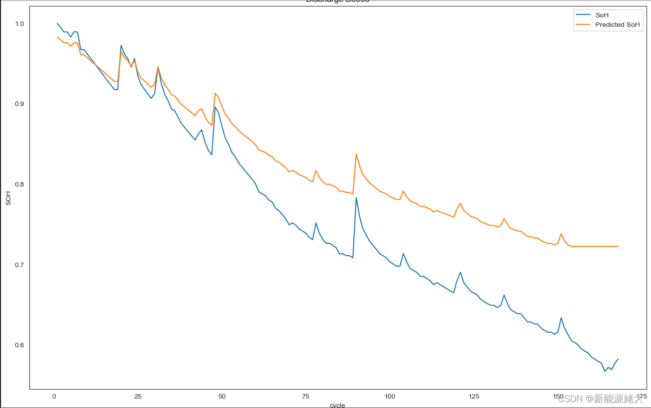
print(dis_ele.head(5))

将实际SOH和神经网络预测的SOH进行对比，并计算均方根误差。

attrib=['capacity', 'voltage_measured', 'current_measured',
        'temperature_measured', 'current_load', 'voltage_load', 'time']
soh_pred = model.predict(sc.fit_transform(dataset_val[attrib]))
print(soh_pred.shape)

C = dataset_val['capacity'][0]
soh = []
for i in range(len(dataset_val)):
  soh.append(dataset_val['capacity'][i] / C)
new_soh = dataset_val.loc[(dataset_val['cycle'] >= 1), ['cycle']]
new_soh['SoH'] =  soh
new_soh['NewSoH'] = soh_pred
new_soh = new_soh.groupby(['cycle']).mean().reset_index()
print(new_soh.head(10))
rms = np.sqrt(mean_squared_error(new_soh['SoH'], new_soh['NewSoH']))
print('Root Mean Square Error: ', rms)

最后，绘制两个SOH的图表，以观察它们的差异。

plot_df = new_soh.loc[(new_soh['cycle']>=1),['cycle','SoH', 'NewSoH']]
sns.set_style("white")
plt.figure(figsize=(16, 10))
plt.plot(plot_df['cycle'], plot_df['SoH'], label='SoH')
plt.plot(plot_df['cycle'], plot_df['NewSoH'], label='Predicted SoH')
#Draw threshold
#plt.plot([0.,len(capacity)], [0.70, 0.70], label='Threshold')
plt.ylabel('SOH')
# make x-axis ticks legible
adf = plt.gca().get_xaxis().get_major_formatter()
plt.xlabel('cycle')
plt.legend()
plt.title('Discharge B0006')

为了估算SOH，可以观察到，数据模式被模型正确地学习，正如理论所预测的那样，因为曲线的形状几乎完全相同。所显示的SOH的行为与预期相同。

估计RUL

与对SOH的估计一样，分别准备了训练和测试的数据集，
使用前50个数据的电池容量数据来预测接下来的循环容量的剩余循环次数。
以便知道电池阈值何时达到。

dataset_val, capacity_val = load_data('B0005')
attrib=['cycle', 'datetime', 'capacity']
dis_ele = capacity_val[attrib]
rows=['cycle','capacity']
dataset=dis_ele[rows]
data_train=dataset[(dataset['cycle']<50)]
data_set_train=data_train.iloc[:,1:2].values
data_test=dataset[(dataset['cycle']>=50)]
data_set_test=data_test.iloc[:,1:2].values

sc=MinMaxScaler(feature_range=(0,1))
data_set_train=sc.fit_transform(data_set_train)
data_set_test=sc.transform(data_set_test)

X_train=[]
y_train=[]
#take the last 10t to predict 10t+1
for i in range(10,49):
    X_train.append(data_set_train[i-10:i,0])
    y_train.append(data_set_train[i,0])
X_train,y_train=np.array(X_train),np.array(y_train)
 
X_train=np.reshape(X_train,(X_train.shape[0],X_train.shape[1],1))

接下来我们进行神经网络的训练。使用LSTM类型的网络，而不是标准的神经网络。

regress = Sequential()
regress.add(LSTM(units=200, return_sequences=True, input_shape=(X_train.shape[1],1)))
regress.add(Dropout(0.3))
regress.add(LSTM(units=200, return_sequences=True))
regress.add(Dropout(0.3))
regress.add(LSTM(units=200, return_sequences=True))
regress.add(Dropout(0.3))
regress.add(LSTM(units=200))
regress.add(Dropout(0.3))
regress.add(Dense(units=1))
regress.compile(optimizer='adam',loss='mean_squared_error')
regress.summary()

X_test=[]
for i in range(10,129):
    X_test.append(inputs[i-10:i,0])
X_test=np.array(X_test)
X_test=np.reshape(X_test,(X_test.shape[0],X_test.shape[1],1))
pred=regress.predict(X_test)
print(pred.shape)
pred=sc.inverse_transform(pred)
pred=pred[:,0]
tests=data_test.iloc[:,1:2]
rmse = np.sqrt(mean_squared_error(tests, pred))
print('Test RMSE: %.3f' % rmse)
metrics.r2_score(tests,pred)

平均RMSE为0.05(5%)，这与文献中使用这种网络观察到的值非常接近。

接下来进行绘图。

ln = len(data_train)
data_test['pre']=pred
plot_df = dataset.loc[(dataset['cycle']>=1),['cycle','capacity']]
plot_per = data_test.loc[(data_test['cycle']>=ln),['cycle','pre']]
plt.figure(figsize=(16, 10))
plt.plot(plot_df['cycle'], plot_df['capacity'], label="Actual data", color='blue')
plt.plot(plot_per['cycle'],plot_per['pre'],label="Prediction data", color='red')
#Draw threshold
plt.plot([0.,168], [1.38, 1.38],dashes=[6, 2], label="treshold")
plt.ylabel('Capacity')
# make x-axis ticks legible
adf = plt.gca().get_xaxis().get_major_formatter()
plt.xlabel('cycle')
plt.legend()
plt.title('Discharge B0005 (prediction) start in cycle 50 -RULe=-8, window-size=10')