EMD经验模态分解为IMF及绘制频谱图

代码如下：

#!/usr/bin/env python3
import pandas as pd
import xlrd
from datetime import *
import matplotlib.pyplot as plt
import numpy as np
from PyEMD import EEMD, EMD, Visualisation
from scipy.signal import hilbert
# from fftlw import fftlw
from vmdpy import VMD


# 分解方法（emd、eemd、vmd）
from xlrd import xldate_as_tuple


#归一化
def normalization(data):
    _range = np.max(data) - np.min(data)
    return (data - np.min(data)) / _range

#EMD去噪
def decompose_lw(signal, method='emd', K=10):
    emd = EMD()
    IMFs = emd.emd(signal)

    signal2 = np.zeros(40551)

    for i in range(np.shape(IMFs)[0] - 2):
        signal2 += IMFs[2 + i, :]
    return signal2


#分解
def decompose_lw1(signal, t, method='emd', K=10):

    emd = EMD()
    IMFs = emd.emd(signal)

    plt.figure()
    for i in range(len(IMFs)):
        plt.subplot(len(IMFs), 1, i + 1)
        plt.plot(t, IMFs[i])
        if i == 0:
            plt.rcParams['font.sans-serif'] = 'Times New Roman'
            plt.title('Decomposition Signal', fontsize=14)
        elif i == len(IMFs) - 1:
            plt.rcParams['font.sans-serif'] = 'Times New Roman'
            plt.xlabel('Time/s')
    #plt.tight_layout()
    # print(IMFs)
    # print(len(IMFs))
    return IMFs

# 希尔波特变换及画时频谱
def hhtlw(IMFs, t,f_range=[0, 500], t_range=[0, 1], ft_size=[128, 128],draw=1):
    fmin, fmax = f_range[0], f_range[1]  # 时频图所展示的频率范围
    tmin, tmax = t_range[0], t_range[1]  # 时间范围
    fdim, tdim = ft_size[0], ft_size[1]  # 时频图的尺寸（分辨率）
    dt = (tmax - tmin) / (tdim - 1)
    df = (fmax - fmin) / (fdim - 1)
    vis = Visualisation()
    # 希尔伯特变化
    c_matrix = np.zeros((fdim, tdim))


    for imf in IMFs:
        imf = np.array([imf])
        # print(imf)
        # 求瞬时频率
        freqs = abs(vis._calc_inst_freq(imf, t, order=False, alpha=None))
        # 求瞬时幅值
        amp = abs(hilbert(imf))
        # 去掉为1的维度
        freqs = np.squeeze(freqs)
        amp = np.squeeze(amp)
        # 转换成矩阵
        temp_matrix = np.zeros((fdim, tdim))
        n_matrix = np.zeros((fdim, tdim))
        for i, j, k in zip(t, freqs, amp):
            if i >= tmin and i <= tmax and j >= fmin and j <= fmax:
                temp_matrix[round((j - fmin) / df)][round((i - tmin) / dt)] += k
                n_matrix[round((j - fmin) / df)][round((i - tmin) / dt)] += 1
        n_matrix = n_matrix.reshape(-1)
        idx = np.where(n_matrix == 0)[0]
        n_matrix[idx] = 1
        n_matrix = n_matrix.reshape(fdim, tdim)
        temp_matrix = temp_matrix / n_matrix
        c_matrix += temp_matrix

    t = np.linspace(tmin, tmax, tdim)
    f = np.linspace(fmin, fmax, fdim)
    # 可视化
    if draw == 1:
        fig, axes = plt.subplots()
        plt.rcParams['font.sans-serif'] = 'Times New Roman'
        plt.contourf(t, f, c_matrix, cmap="jet")
        plt.xlabel('Time/s', fontsize=16)
        plt.ylabel('Frequency/Hz', fontsize=16)
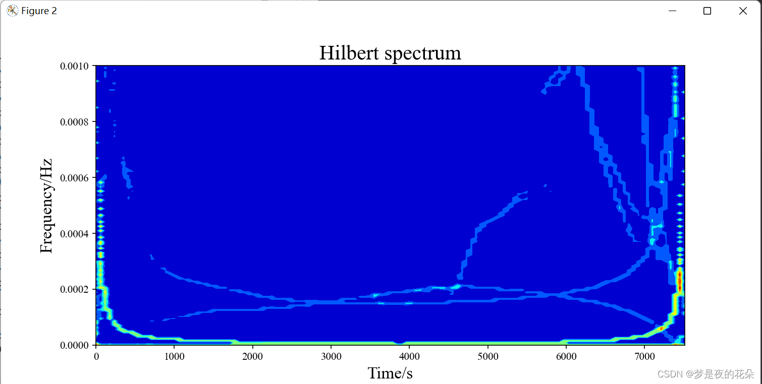
        plt.title('Hilbert spectrum', fontsize=20)
        x_labels = axes.get_xticklabels()
        [label.set_fontname('Times New Roman') for label in x_labels]
        y_labels = axes.get_yticklabels()
        [label.set_fontname('Times New Roman') for label in y_labels]
        plt.show()
    return t, f, c_matrix


# %%测试函数
if __name__ == '__main__':
    # 构造测试信号
    t = np.arange(0, 40551, 1.0)
    wb = xlrd.open_workbook("D:\yanfiles\石油工程数据分析与数据挖掘课题组\data\实验data\保-平25井4+5#压裂秒钟报表.xlsx")
    sheet = wb.sheet_by_index(0)  #获取第一个sheet页
    signal = sheet.col_values(0) #获取第一列数据
    signal1 = normalization(signal)
    signal2 = decompose_lw(signal1)
    plt.figure()
    plt.plot(t, signal2)
    plt.rcParams['font.sans-serif'] = 'Times New Roman'
    plt.xlabel('Time/s', fontsize=16)
    plt.title('Original Signal', fontsize=20)
    plt.show()

    # 画仿真信号频谱图
    # _,_=fftlw(Fs,signal,1)
    # IMFs = decompose_lw(signal, t, method='vmd', K=10)  # 分解信号
    IMFs = decompose_lw1(np.array(signal2), t)  # 未去噪分解信号
    tt, ff, c_matrix = hhtlw(IMFs, t, f_range=[0, 0.001], t_range=[0,40551], ft_size=[128, 128])  # 画希尔伯特谱

• 原始时间序列

• 分解为IMFs
  
• 频谱图希尔伯特谱