《吴恩达深度学习》浅层神经网络作业(python版)
本版本就是根据吴恩达作业提供的指导思路完成的。
1. load data
花瓣数据的极坐标方程通常为 r(θ)=acos(kθ)r(θ)=acos(kθ) 或 r(θ)=asin(kθ)r(θ)=asin(kθ)。其中,kk是整数,决定了花瓣的数量。当 k 为奇数时,曲线将有 kk 个花瓣;当 k为偶数时,曲线将有 2k个花瓣
import matplotlib.pyplot as plt
import numpy as np
import sklearn
import sklearn.datasets
import sklearn.linear_model

def load_planar_dataset():
    np.random.seed(1)
    m = 400 # number of examples
    N = int(m/2) # number of points per class
    D = 2 # dimensionality
    X = np.zeros((m,D)) # data matrix where each row is a single example
    Y = np.zeros((m,1), dtype='uint8') # labels vector (0 for red, 1 for blue)
    a = 4 # maximum ray of the flower

    for j in range(2):
        ix = range(N*j,N*(j+1))
        t = np.linspace(j*3.12,(j+1)*3.12,N) + np.random.randn(N)*0.2 # theta
        r = a*np.sin(4*t) + np.random.randn(N)*0.2 # radius
        X[ix] = np.c_[r*np.sin(t), r*np.cos(t)]
        Y[ix] = j

    X = X.T
    Y = Y.T

    return X, Y
2. 回归函数
def sigmoid(x):

    s = 1/(1+np.exp(-x))
    return s
3.初始化参数
X,Y = load_planar_dataset()
n_x = X.shape[0] # size of input layer
n_h = 4
n_y = Y.shape[0] # size of output layer
def initialize_parameters(n_x, n_h, n_y):
    np.random.seek(2)
    W1 = np.random.randn(n_h,n_x)*0.01
    b1 = np.zeros((n_h,1))
    W2 = np.random.randn(n_y,n_h)*0.01
    b2 = np.zeros((n_y,1))
    assert (W1.shape == (n_h, n_x))
    assert (b1.shape == (n_h, 1))
    assert (W2.shape == (n_y, n_h))
    assert (b2.shape == (n_y, 1))

    parameters = {"W1": W1,
                  "b1": b1,
                  "W2": W2,
                  "b2": b2}
    return parameters
4.向前传播->代价函数->向后传播
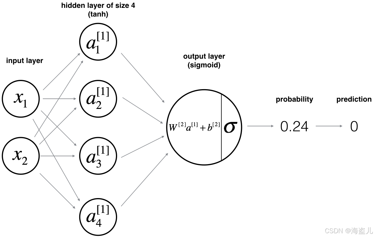
def forward_propagation(X, parameters):
    W1 = parameters["W1"]
    b1 = parameters["b1"]
    W2 = parameters["W2"]
    b2 = parameters["b2"]

    Z1 = W1@X + b1
    A1 = np.tanh(Z1)
    Z2 = W2@A1 + b2
    A2 = sigmoid(Z2)

    assert(A2.shape == (1, X.shape[1]))

    cache = {"Z1": Z1,
             "A1": A1,
             "Z2": Z2,
             "A2": A2}
    return A2, cache
def compute_cost(A2, Y, parameters):
m = Y.shape[1]
logprobs = np.dot(np.log(A2),Y.T) + np.dot(np.log(1-A2),(1-Y).T)
cost = -(logprobs).sum()/m
assert(isinstance(cost, float))
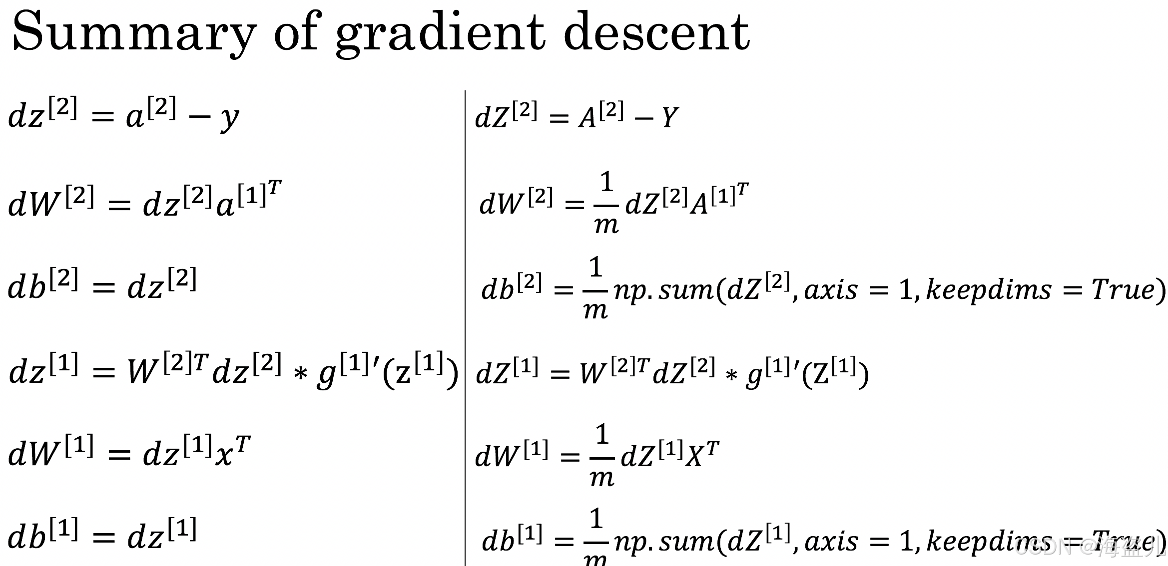
return costdef back_prapagation(parameters, cache, X, Y):
W1 = parameters["W1"]
W2 = parameters["W2"]
A1 = cache["A1"]
A2 = cache["A2"]
m = X.shape[1]
dZ2 = A2 - Y
dW2 = np.dot(dZ2, A1.T)/m
db2 = np.sum(dZ2, axis=1,keepdims=True)/m
dZ1 = (np.dot(W2.T, dZ2))*(1-np.power(A1,2))
dW1 = np.dot(dZ1, X.T)/m
db1 = np.sum(dZ1,axis=1,keepdims=True)/m
grads = {"dW1": dW1,
"db1": db1,
"dW2": dW2,
"db2": db2}
return grads5.更新参数
def update_parameters(parameters, grads, learning_rate=1.2):
    W1 = parameters["W1"]
    b1 = parameters["b1"]
    W2 = parameters["W2"]
    b2 = parameters["b2"]

    dW1 = grads["dW1"]
    db1 = grads["db1"]
    dW2 = grads["dW2"]
    db2 = grads["db2"]

    W1 = W1-learning_rate*dW1
    b1 = b1-learning_rate*db1
    W2 = W2-learning_rate*dW2
    b2 = b2-learning_rate*db2

    parameters = {"W1": W1,
                  "b1": b1,
                  "W2": W2,
                  "b2": b2}

    return parameters
6.组成模型
def nn_model(X, Y, n_h, num_iterations = 10000, print_cost=False):
    np.random.seed(3)

    parameters = initialize_parameters(n_x, n_h, n_y)
    W1 = parameters["W1"]
    b1 = parameters["b1"]
    W2 = parameters["W2"]
    b2 = parameters["b2"]
    for i in range(0, num_iterations):
        A2, cache = forward_propagation(X, parameters)
        cost = compute_cost(A2, Y , parameters)
        grads = back_prapagation(parameters, cache, X, Y)
        parameters = update_parameters(parameters, grads)
        if print_cost and i % 1000 == 0:
            print ("Cost after iteration %i: %f" %(i, cost))
    return parameters
def predict(parameters, X):
    A2, cache = forward_propagation(X,parameters)
    predictions = A2>0.5

    return predictions
7.预测结果和图形绘制
parameters = nn_model(X, Y, n_h = 4, num_iterations = 10000, print_cost=True)
# Plot the decision boundary
def plot_decision_boundary(model, X, y):
# Set min and max values and give it some padding
x_min, x_max = X[0, :].min() - 1, X[0, :].max() + 1
y_min, y_max = X[1, :].min() - 1, X[1, :].max() + 1
h = 0.01
# Generate a grid of points with distance h between them
xx, yy = np.meshgrid(np.arange(x_min, x_max, h), np.arange(y_min, y_max, h))
# Predict the function value for the whole grid
Z = model(np.c_[xx.ravel(), yy.ravel()])
Z = Z.reshape(xx.shape)
# Plot the contour and training examples
plt.contourf(xx, yy, Z, cmap=plt.cm.Spectral)
plt.ylabel('x2')
plt.xlabel('x1')
plt.scatter(X[0, :], X[1, :], c=y, cmap=plt.cm.Spectral)
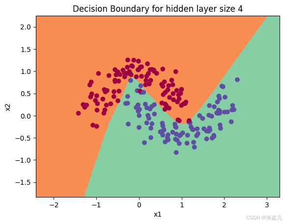
plot_decision_boundary(lambda x: predict(parameters, x.T), X, Y)
plt.title("Decision Boundary for hidden layer size " + str(4))Cost after iteration 0: 0.693048
Cost after iteration 1000: 0.288083
Cost after iteration 2000: 0.254385
Cost after iteration 3000: 0.233864
Cost after iteration 4000: 0.226792
Cost after iteration 5000: 0.222644
Cost after iteration 6000: 0.219731
Cost after iteration 7000: 0.217504
Cost after iteration 8000: 0.219573
Cost after iteration 9000: 0.218590
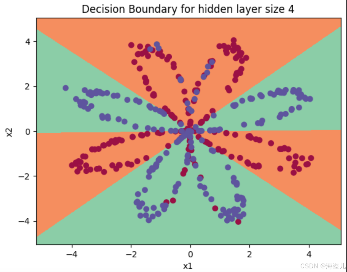
predictions = predict(parameters, X)
print ('Accuracy: %d' % float((np.dot(Y,predictions.T) + np.dot(1-Y,1-predictions.T))/float(Y.size)*100) + '%')
Accuracy: 90%
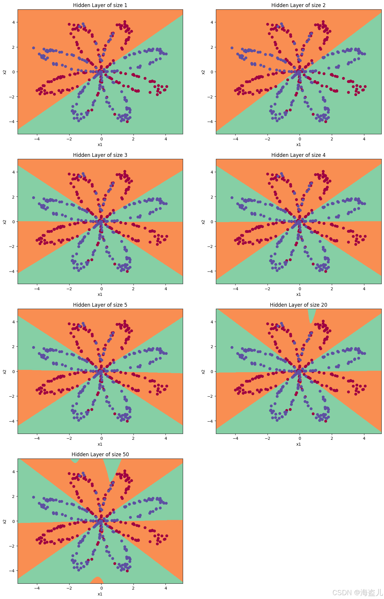
8. 隐藏层不同size导致的结果影响
plt.figure(figsize=(16, 32))
hidden_layer_sizes = [1, 2, 3, 4, 5, 20, 50]
for i, n_h in enumerate(hidden_layer_sizes):
    plt.subplot(5, 2, i+1)
    plt.title('Hidden Layer of size %d' % n_h)
    parameters = nn_model(X, Y, n_h, num_iterations = 5000)
    plot_decision_boundary(lambda x: predict(parameters, x.T), X, Y)
    predictions = predict(parameters, X)
    accuracy = float((np.dot(Y,predictions.T) + np.dot(1-Y,1-predictions.T))/float(Y.size)*100)
    print ("Accuracy for {} hidden units: {} %".format(n_h, accuracy))
Accuracy for 1 hidden units: 67.5 %
Accuracy for 2 hidden units: 67.25 %
Accuracy for 3 hidden units: 90.75 %
Accuracy for 4 hidden units: 90.5 %
Accuracy for 5 hidden units: 91.25 %
Accuracy for 20 hidden units: 90.5 %
Accuracy for 50 hidden units: 90.75 %
9. 其他dataset测试
def load_extra_datasets():
    N = 200
    noisy_circles = sklearn.datasets.make_circles(n_samples=N, factor=.5, noise=.3)
    noisy_moons = sklearn.datasets.make_moons(n_samples=N, noise=.2)
    blobs = sklearn.datasets.make_blobs(n_samples=N, random_state=5, n_features=2, centers=6)
    gaussian_quantiles = sklearn.datasets.make_gaussian_quantiles(mean=None, cov=0.5, n_samples=N, n_features=2, n_classes=2, shuffle=True, random_state=None)
    no_structure = np.random.rand(N, 2), np.random.rand(N, 2)

    return noisy_circles, noisy_moons, blobs, gaussian_quantiles, no_structure

# Datasets
noisy_circles, noisy_moons, blobs, gaussian_quantiles, no_structure = load_extra_datasets()

datasets = {"noisy_circles": noisy_circles,
            "noisy_moons": noisy_moons,
            "blobs": blobs,
            "gaussian_quantiles": gaussian_quantiles}

### START CODE HERE ### (choose your dataset)
dataset = "noisy_moons"
### END CODE HERE ###

X, Y = datasets[dataset]
X, Y = X.T, Y.reshape(1, Y.shape[0])

plt.scatter(X[0, :], X[1, :], c=Y, s=40, cmap=plt.cm.Spectral);
plt.show()


parameters = nn_model(X, Y, n_h = 4, num_iterations = 10000, print_cost=True)


# Plot the decision boundary
plot_decision_boundary(lambda x: predict(parameters, x.T), X, Y)
plt.title("Decision Boundary for hidden layer size " + str(4))
# make blobs binary
if dataset == "blobs":
    Y = Y%2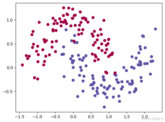
知识点之plt.contourf
plt.contourf(xx, yy, Z, cmap=plt.cm.Spectral) 是 Matplotlib 中用于绘制填充等高线图的函数。它的作用是根据输入的网格数据和对应的值,用颜色填充不同区域的等高线,直观展示二维数据的分布或分类结果。以下是各参数的解释:
参数说明
xx和yy
由
numpy.meshgrid生成的二维网格坐标矩阵,表示平面上所有点的横纵坐标。例如:如果原始数据是
x和y两个一维数组,xx, yy = np.meshgrid(x, y)会生成覆盖整个平面的网格点。
Z
与
xx和yy形状相同的二维数组,表示每个网格点对应的数值(如分类概率、函数值等)。例如:在分类问题中,
Z可以是模型对每个点的预测结果(类别或概率)。
cmap=plt.cm.Spectral
指定颜色映射(colormap),这里使用
Spectral色系,特点是彩虹色渐变(红→橙→黄→绿→蓝→紫)。适合高对比度可视化,但需注意:在黑白打印或色觉障碍场景中可能不友好(可用
viridis等替代)。
-
分类决策边界可视化
在机器学习中,常结合contourf绘制分类模型的决策区域,用不同颜色区分各类别区域。python
复制
# 示例:绘制 SVM 分类结果
h = 0.02  # 网格步长
x_min, x_max = X[:, 0].min() - 1, X[:, 0].max() + 1
y_min, y_max = X[:, 1].min() - 1, X[:, 1].max() + 1
xx, yy = np.meshgrid(np.arange(x_min, x_max, h), np.arange(y_min, y_max, h))
Z = model.predict(np.c_[xx.ravel(), yy.ravel()])  # 模型预测每个网格点
Z = Z.reshape(xx.shape)
plt.contourf(xx, yy, Z, cmap=plt.cm.Spectral)
plt.scatter(X[:,0], X[:,1], c=y, cmap=plt.cm.Spectral)  # 叠加原始数据点

腾讯云面向开发者汇聚海量精品云计算使用和开发经验,营造开放的云计算技术生态圈。
更多推荐
 3
3 0
0- 0


 已为社区贡献6条内容

所有评论(0)