Python/torch/深度学习——UNet学习记录

---

---

前言

主要用于记录UNet学习过程，随时可能修改。

---

一、UNet模型源码

torch库下的UNet模型源码（本来用GPT写，但是不得不说GPT写的跳跃连接有点毛病，最后还是自己写了）
代码已经经过了测试，运行没有问题，其中包含了点nnUNet对原模型做的修改（未测试）
这里与源码不一样的是DoubleConv中，卷积层添加了padding=1，padding_mode=‘reflect’，bias=False
主要是为了让图片不缩放（好像影响不大，调试的时候挺友好的）

transforms = torchvision.transforms.Compose([
    torchvision.transforms.ToTensor()]
)


class DoubleConv(nn.Module):
    def __init__(self, in_channels, out_channels):
        super(DoubleConv, self).__init__()
        self.block = nn.Sequential(
            nn.Conv2d(in_channels, out_channels, kernel_size=3, padding=1,
                      stride=1, padding_mode='reflect', bias=False),

            nn.BatchNorm2d(out_channels),
            # nn.InstanceNorm2d(out_channels),  # nnUNet

            nn.ReLU(inplace=True),
            # nn.LeakyReLU(),  # nnUNet

            nn.Conv2d(out_channels, out_channels, kernel_size=3, padding=1,
                      stride=1, padding_mode='reflect', bias=False),

            nn.BatchNorm2d(out_channels),
            # nn.InstanceNorm2d(out_channels),  # nnUNet

            nn.ReLU(inplace=True)
            # nn.LeakyReLU()  # nnUNet
        )

    def forward(self, x):
        return self.block(x)


# class DownSample(nn.Module):
#     def __init__(self, in_channels, out_channels):
#         super(DownSample, self).__init__()
#         self.block = nn.Sequential(
#             DoubleConv(in_channels, out_channels),
#             nn.MaxPool2d(kernel_size=2, stride=2)
#         )
# 
#     def forward(self, x):
#         return self.block(x)



class UpSample(nn.Module):
    def __init__(self, in_channels, out_channels):
        super(UpSample, self).__init__()
        self.block = nn.Sequential(
            nn.ConvTranspose2d(in_channels, in_channels//2, kernel_size=2, stride=2),
            # nn.Conv2d(in_channels//2, out_channels, kernel_size=1, stride=1)
            DoubleConv(in_channels//2, out_channels)
        )

    def forward(self, x):
        return self.block(x)


# 定义UNet模型
class UNet(nn.Module):
    def __init__(self, in_channels=3, out_channels=3):
        super().__init__()
        self.conv1 = DoubleConv(in_channels, 64)
        self.down1 = nn.MaxPool2d(kernel_size=2, stride=2)
        self.conv2 = DoubleConv(64, 128)
        self.down2 = nn.MaxPool2d(kernel_size=2, stride=2)
        self.conv3 = DoubleConv(128, 256)
        self.down3 = nn.MaxPool2d(kernel_size=2, stride=2)
        self.conv4 = DoubleConv(256, 512)
        self.down4 = nn.MaxPool2d(kernel_size=2, stride=2)

        self.conv_mid = DoubleConv(512, 1024)

        self.up1 = nn.ConvTranspose2d(1024, 512, kernel_size=2, stride=2)
        self.up_conv1 = DoubleConv(1024, 512)
        self.up2 = nn.ConvTranspose2d(512, 256, kernel_size=2, stride=2)
        self.up_conv2 = DoubleConv(512, 256)
        self.up3 = nn.ConvTranspose2d(256, 128, kernel_size=2, stride=2)
        self.up_conv3 = DoubleConv(256, 128)
        self.up4 = nn.ConvTranspose2d(128, 64, kernel_size=2, stride=2)
        self.up_conv4 = DoubleConv(128, 64)

        self.out_channel = nn.Conv2d(64, out_channels, kernel_size=1, stride=1)

        self.sigmoid = nn.Sigmoid()

    def forward(self, x):
        conv1 = self.conv1(x)
        down1 = self.down1(conv1)
        conv2 = self.conv2(down1)
        down2 = self.down2(conv2)
        conv3 = self.conv3(down2)
        down3 = self.down3(conv3)
        conv4 = self.conv4(down3)
        down4 = self.down4(conv4)

        conv_mid = self.conv_mid(down4)

        up1 = self.up1(conv_mid)
        cat1 = torch.cat([up1, conv4], dim=1)
        up_conv1 = self.up_conv1(cat1)

        up2 = self.up2(up_conv1)
        cat2 = torch.cat([up2, conv3], dim=1)
        up_conv2 = self.up_conv2(cat2)

        up3 = self.up3(up_conv2)
        cat3 = torch.cat([up3, conv2], dim=1)
        up_conv3 = self.up_conv3(cat3)

        up4 = self.up4(up_conv3)
        cat4 = torch.cat([up4, conv1], dim=1)
        up_conv4 = self.up_conv4(cat4)

        out_channel = self.out_channel(up_conv4)
        out = self.sigmoid(out_channel)
        return out```

---

二、模型结构

1.UNet模型

UNet模型结构图：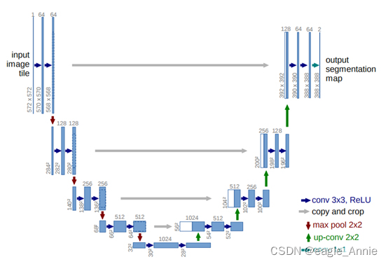

简单理解一下：
1、4层编码（DoubleConv - MaxPool2d）
（MaxPool2d才是下采样，这里更正一下）
2、双层卷积（DoubleConv）
3-1、4层解码（ConvTranspose2d - DoubleConv）
（ConvTranspose2d 是上采样的一种方式，这里更正一下）
3-2、上采样的同时，torch.cat 4层编码中的结果
（注意这里是DoubleConv 出来的，不是MaxPool2d后的！！）
（torch.cat是将图像拼在后面，add是加在一起，两者图像数量不同）
（也叫跳跃连接）
5、输出层（2分类，语义分割本质还是分类，label中图五颜六色的还是分类，无非不是出数组，是出图了而已）

---

三、模型代码解释

1.双层卷积

因为多处用到：
Conv2d卷积——BN——ReLU激活函数——Conv2d卷积——BN——ReLU激活函数
这里独立定义一个DoubleConv类（2层Conv2d+2层BN+2层ReLU），方便调用

class DoubleConv(nn.Module):
    def __init__(self, in_channels, out_channels):
        super(DoubleConv, self).__init__()
        self.block = nn.Sequential(
            nn.Conv2d(in_channels, out_channels, kernel_size=3, padding=1,
                      stride=1, padding_mode='reflect', bias=False),

            nn.BatchNorm2d(out_channels),
            # nn.InstanceNorm2d(out_channels),  # nnUNet

            nn.ReLU(inplace=True),
            # nn.LeakyReLU(),  # nnUNet

            nn.Conv2d(out_channels, out_channels, kernel_size=3, padding=1,
                      stride=1, padding_mode='reflect', bias=False),

            nn.BatchNorm2d(out_channels),
            # nn.InstanceNorm2d(out_channels),  # nnUNet

            nn.ReLU(inplace=True)
            # nn.LeakyReLU()  # nnUNet
        )

    def forward(self, x):
        return self.block(x)

---

2.编码

下采样有池化法和卷积法：
采用stride为2的池化层，如Max-pooling（最大池化）和Average-pooling（平均池化）
Max-pooling：计算简单，能够更好的保留纹理特征（相比平均池化）
但是池化层是不可学习的，因此使用卷积层能带来更好的效果，但也会增加计算量；一般使用都会将两者结合。

这里4个编码分开写了，测试中才发现 torch.cat 用的是conv1、2、3、4的结果，踩了个坑
DoubleConv 和 MaxPool2d 组成1个编码。
1个编码结构实际为：
Conv2d——BN——ReLU——Conv2d——BN——ReLU——MaxPool2d
在 MaxPool2d 这一步后才缩减了图片尺寸，DoubleConv设置只改变通道数

        # class UNet中的
        self.conv1 = DoubleConv(in_channels, 64)
        self.down1 = nn.MaxPool2d(kernel_size=2, stride=2)
        self.conv2 = DoubleConv(64, 128)
        self.down2 = nn.MaxPool2d(kernel_size=2, stride=2)
        self.conv3 = DoubleConv(128, 256)
        self.down3 = nn.MaxPool2d(kernel_size=2, stride=2)
        self.conv4 = DoubleConv(256, 512)
        self.down4 = nn.MaxPool2d(kernel_size=2, stride=2)

---

3.解码

上采样可以将一个低分辨率的图像还原成一个高分辨率的图像，常用的方法有双线性插值法，反卷积（也称转置卷积）法和上池化法；根据代码来看，UNet所采用的的是反卷积法。
ConvTranspose2d定义了一个转置卷积层，用于反卷积。
参考链接

这里直接定义了1个解码
ConvTranspose2d 和 DoubleConv 组成1个解码。
1个解码结构实际为：
ConvTranspose2d——Conv2d——BN——ReLU——Conv2d——BN——ReLU

class UpSample(nn.Module):
    def __init__(self, in_channels, out_channels):
        super(UpSample, self).__init__()
        self.block = nn.Sequential(
            nn.ConvTranspose2d(in_channels, in_channels//2, kernel_size=2, stride=2),
            # nn.Conv2d(in_channels//2, out_channels, kernel_size=1, stride=1)
            DoubleConv(in_channels//2, out_channels)
        )

    def forward(self, x):
        return self.block(x)

---

三、损失函数选择

训练 U-Net 网络时，根据具体任务和数据的性质，可以使用多种损失函数。损失函数的选择取决于具体任务和数据的特征， 以下是U-Net的一些常用损失函数。4-5目前基本没见过，就留个坑先。

1.Binary Cross Entropy (BCE) Loss

• 交叉熵损失函数，通常用于二元分割任务，即目标值只有两个类别，其中每个像素被分类为前景或背景。
• 输入数据应该是0或1的概率，代表两个类别的预测概率（一般是sigmoid后的参数）
• BCELoss对每个样本计算的是二元交叉熵损失，然后对所有样本的损失取平均值。

CrossEntropyLoss（补充对比）

• 交叉熵损失函数，适用于多分类问题，即目标值有多个类别。
• 输入数据是未经过softmax处理的原始预测值，是一个包含各类别分数的向量（一般对应softmax，但是输入为softmax前的数据，这里与BCELoss不同，因为CrossEntropyLoss已经包含了softmax）
• CrossEntropyLoss对每个样本的预测值进行softmax操作得到概率分布，然后计算多类交叉熵损失，最后对所有样本的损失取平均值。

---

2.Dice Loss

Dice Loss（Dice 损失）是图像分割任务的另一种流行选择，用于测量预测分割和背景之间的重叠。 Dice 系数的范围为 0 到 1，其中 1 表示完美重叠。
这个和IOU（预测结果的与 label 的交集/预测结果的与 label 的并集）非常像，两者的区别在于计算方式不同；Dice对 predict（预测结果）与 label（标签）的交集和并集的贡献是相等的，而IOU更加关注 predict（预测结果）与 label（标签）的交集。因此，Dice系数更加敏感于小目标，而IOU则更加适用于大目标的检测和分割任务。
$$Dice=2\ast TP/(2\ast TP+FP+FN)=(TP+TP)/((TP+TP)+FP+FN）$$
$$DiceLoss=1-Dice$$
$$IOU=TP/(TP+FP+FN)$$
TP（True Positive）表示预测为正样本且标签为正样本的像素数量，FP（False Positive）表示预测为正样本但标签为负样本的像素数量，FN（False Negative）表示预测为负样本但标签为正样本的像素数量。Dice系数的取值范围在0到1之间，其值越接近1，表示预测结果与真实标签的重叠度越高，相似度越高。

Dice Loss这个在torch库中是没有的，需要自己写函数段

import torch
from torch import Tensor


def dice_coeff(input: Tensor, target: Tensor, reduce_batch_first: bool = False, epsilon=1e-6):
    # Average of Dice coefficient for all batches, or for a single mask
    assert input.size() == target.size()
    if input.dim() == 2 and reduce_batch_first:
        raise ValueError(f'Dice: asked to reduce batch but got tensor without batch dimension (shape {input.shape})')

    if input.dim() == 2 or reduce_batch_first:
        inter = torch.dot(input.reshape(-1), target.reshape(-1))
        sets_sum = torch.sum(input) + torch.sum(target)
        if sets_sum.item() == 0:
            sets_sum = 2 * inter

        return (2 * inter + epsilon) / (sets_sum + epsilon)
    else:
        # compute and average metric for each batch element
        dice = 0
        for i in range(input.shape[0]):
            dice += dice_coeff(input[i, ...], target[i, ...])
        return dice / input.shape[0]


def multiclass_dice_coeff(input: Tensor, target: Tensor, reduce_batch_first: bool = False, epsilon=1e-6):
    # Average of Dice coefficient for all classes
    assert input.size() == target.size()
    dice = 0
    for channel in range(input.shape[1]):
        dice += dice_coeff(input[:, channel, ...], target[:, channel, ...], reduce_batch_first, epsilon)

    return dice / input.shape[1]


def dice_loss(input: Tensor, target: Tensor, multiclass: bool = False):
    # Dice loss (objective to minimize) between 0 and 1
    assert input.size() == target.size()
    fn = multiclass_dice_coeff if multiclass else dice_coeff
    return 1 - fn(input, target, reduce_batch_first=True)

---

3.Jaccard Loss (Intersection over Union, IoU)

用于衡量预测分割与真实数据之间的相似度，也是作为语义分割模型评价标准用的比较多的。 具体介绍见Dice Loss。
$$IOU=预测结果的与label的交集/预测结果的与label的并集$$
也就是
$$IOU=TP/(TP+FP+FN)$$

4.Focal Loss

焦点损失（Focal Loss）旨在解决分割任务中的类别不平衡问题。 它为难以分类的像素分配更高的权重，这有助于将训练集中在具有挑战性的区域。

5.Generalized Dice Loss

广义 Dice 损失是导致类别不平衡的 Dice 损失的延伸。 它分别计算每个类别的 Dice 系数，然后使用加权平均值将它们组合起来。