前言

系列专栏:【深度学习：算法项目实战】✨︎
涉及医疗健康、财经金融、商业零售、食品饮料、运动健身、交通运输、环境科学、社交媒体以及文本和图像处理等诸多领域，讨论了各种复杂的深度神经网络思想，如卷积神经网络、循环神经网络、生成对抗网络、门控循环单元、长短期记忆、自然语言处理、深度强化学习、大型语言模型和迁移学习。

本文旨在使用Keras等深度学习库，并熟悉神经网络的基础。

1. 数据集介绍

您可以从免费提供的UCI机器学习存储库中找到葡萄酒质量数据集。数据集由数据中包含的 12 个变量组成。其中少数如下——

• 固定酸度： 总酸度分为两组：挥发性酸和非挥发性或固定酸。此变量的值在数据集中以 gm/dm3 表示。
• 挥发性酸度： 挥发性酸度是葡萄酒变成醋的过程。在该数据集中，挥发性酸度以 gm/dm3 表示。
• 柠檬酸： 柠檬酸是葡萄酒中的固定酸之一。它在数据集中以 g/dm3 表示。
• 残糖： 残糖是发酵停止或停止后剩余的糖。它在数据集中以 g/dm3 表示。
• 氯化物： 它可能是葡萄酒咸味的重要因素。此变量的值在数据集中以 gm/dm3 表示。
• 游离二氧化硫： 它是添加到葡萄酒中的二氧化硫的一部分。此变量的值在数据集中以 gm/dm3 表示。
• 总二氧化硫： 它是结合二氧化硫和游离二氧化硫的总和。此变量的值在数据集中以 gm/dm3 表示。

1.1 获取数据

# Import Required Libraries
import numpy as np
import pandas as pd
import matplotlib.pyplot as plt

# Read in white wine data
white = pd.read_csv("http://archive.ics.uci.edu/ml/machine-learning-databases/wine-quality/winequality-white.csv", sep =';')

# Read in red wine data
red = pd.read_csv("http://archive.ics.uci.edu/ml/machine-learning-databases/wine-quality/winequality-red.csv", sep =';')

1.2 红酒前五行数据

# First rows of `red`
red.head()

输出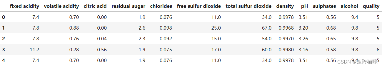

1.3 白酒末五行数据

# Last rows of `white`
white.tail()

输出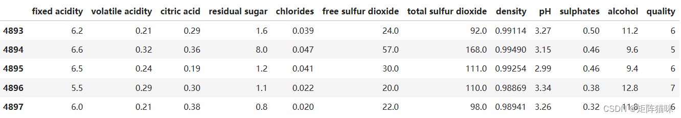

取五行红酒的数据样本

# Take a sample of five rows of `red`
red.sample(5)

输出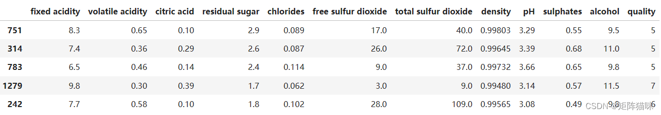

1.4 数据描述

# Describe `white`
white.describe()

输出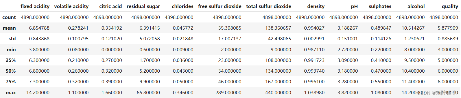

1.5 检查红酒中的空值

# Double check for null values in `red`
pd.isnull(red)

输出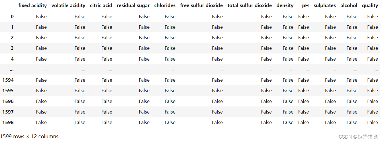

2. 酒精的分布（可视化探索性分析）

2.1 创建直方图

# Create Histogram
fig, ax = plt.subplots(1, 2)

ax[0].hist(red.alcohol, 10, facecolor ='red',
			alpha = 0.5, label ="Red wine")

ax[1].hist(white.alcohol, 10, facecolor ='white',
		ec ="black", lw = 0.5, alpha = 0.5,
		label ="White wine")

fig.subplots_adjust(left = 0, right = 1, bottom = 0, 
			top = 0.5, hspace = 0.05, wspace = 1)

ax[0].set_ylim([0, 1000])
ax[0].set_xlabel("Alcohol in % Vol")
ax[0].set_ylabel("Frequency")
ax[1].set_ylim([0, 1000])
ax[1].set_xlabel("Alcohol in % Vol")
ax[1].set_ylabel("Frequency")

fig.suptitle("Distribution of Alcohol in % Vol")
plt.show()

输出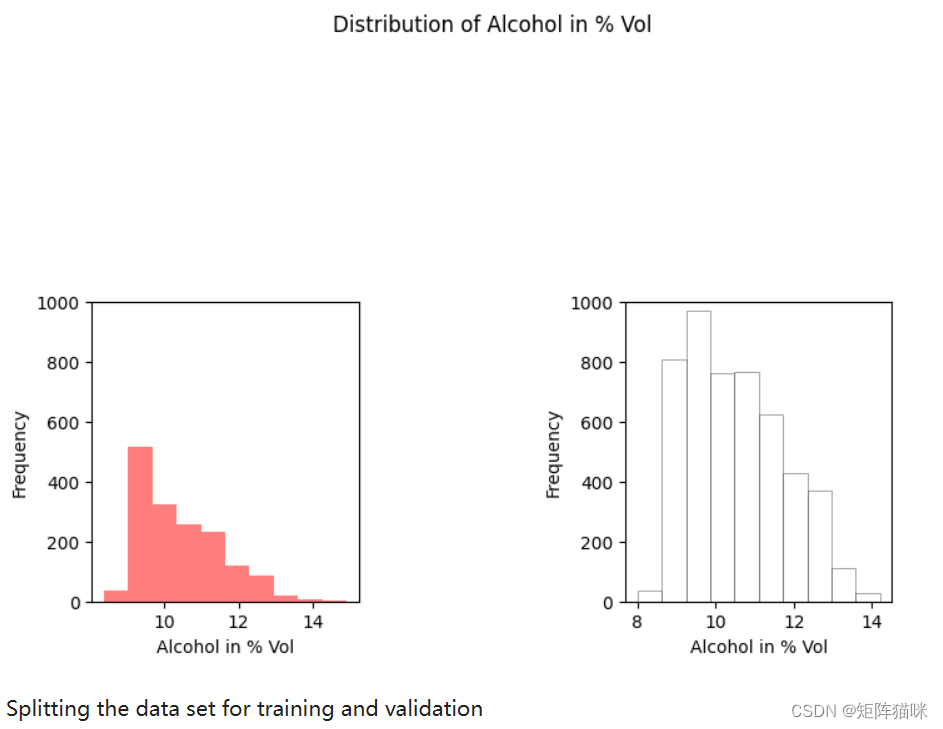

2.2 拆分数据集来进行训练和验证

# Add `type` column to `red` with price one
red['type'] = 1

# Add `type` column to `white` with price zero
white['type'] = 0

# Concat `white` with `red`
wines = pd.concat([red,white], ignore_index = True)

# Import `train_test_split` from `sklearn.model_selection`
from sklearn.model_selection import train_test_split
X = wines.iloc[:, 0:11]
y = np.ravel(wines.type)

# Splitting the data set for training and validating 
X_train, X_test, y_train, y_test = train_test_split(
		X, y, test_size = 0.34, random_state = 45)

3. 创建神经网络模型

3.1 定义网络结构

# Initialize the constructor
model = Sequential()
model.add(Input(shape = (11, )))
model.add(Dense(16, activation ='relu'))
model.add(Dense(8, activation ='relu'))
model.add(Dense(1, activation ='sigmoid'))

# Model config
model.get_config()

# List all weight tensors
model.get_weights()

3.2 定义损失与优化器

model.compile(loss ='binary_crossentropy', optimizer ='adam', metrics =['accuracy'])

model.summary()

Model: "sequential"
┏━━━━━━━━━━━━━━━━━━━━━━━━━━━━━━━━━━━━━━┳━━━━━━━━━━━━━━━━━━━━━━━━━━━━━┳━━━━━━━━━━━━━━━━━┓
┃ Layer (type)                         ┃ Output Shape                ┃         Param # ┃
┡━━━━━━━━━━━━━━━━━━━━━━━━━━━━━━━━━━━━━━╇━━━━━━━━━━━━━━━━━━━━━━━━━━━━━╇━━━━━━━━━━━━━━━━━┩
│ dense (Dense)                        │ (None, 16)                  │             192 │
├──────────────────────────────────────┼─────────────────────────────┼─────────────────┤
│ dense_1 (Dense)                      │ (None, 8)                   │             136 │
├──────────────────────────────────────┼─────────────────────────────┼─────────────────┤
│ dense_2 (Dense)                      │ (None, 1)                   │               9 │
└──────────────────────────────────────┴─────────────────────────────┴─────────────────┘
 Total params: 337 (1.32 KB)
 Trainable params: 337 (1.32 KB)
 Non-trainable params: 0 (0.00 B)

4. 模型训练

# Training Model
history = model.fit(X_train, y_train, epochs = 50, batch_size = 10, verbose = 1, validation_data = (X_test, y_test))

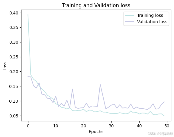
4.1 绘制Loss曲线

history_df = pd.DataFrame(history.history)

plt.plot(history_df.loc[:, ['loss']], "#BDE2E2", label='Training loss')
plt.plot(history_df.loc[:, ['val_loss']],"#C2C4E2", label='Validation loss')
plt.title('Training and Validation loss')
plt.xlabel('Epochs')
plt.ylabel('Loss')
plt.legend(loc="best")

plt.show()

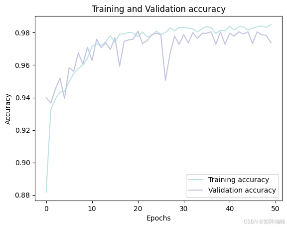
4.2 绘制Accuracy曲线

history_df = pd.DataFrame(history.history)

plt.plot(history_df.loc[:, ['accuracy']], "#BDE2E2", label='Training accuracy')
plt.plot(history_df.loc[:, ['val_accuracy']], "#C2C4E2", label='Validation accuracy')

plt.title('Training and Validation accuracy')
plt.xlabel('Epochs')
plt.ylabel('Accuracy')
plt.legend()
plt.show()

5. 模型评估

计算测试集的预测结果

# Predicting the test set results
predictions_prob = model.predict(X_test)
predictions = (predictions_prob > 0.5)

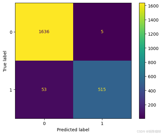
5.1 绘制混淆矩阵

cf_matrix = confusion_matrix(y_test, predictions)
disp = ConfusionMatrixDisplay(confusion_matrix=cf_matrix,)
disp.plot()

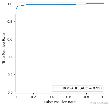
5.2 绘制ROC-AUC曲线

# 计算FPR, TPR, thresholds
fpr, tpr, thresholds = roc_curve(y_test, predictions_prob)
# 计算AUC值
roc_auc = auc(fpr, tpr)
display = RocCurveDisplay(fpr=fpr, tpr=tpr, roc_auc=roc_auc,
                          estimator_name='ROC-AUC')
display.plot()

相关文章

1. 基于前馈神经网络FNN实现葡萄酒类型分类Acc99%(PyTorch版)
2. 基于K-近邻(KNN)、高斯贝叶斯(GaussianNB)、SVC、随机森林(RF)、梯度提升树(GBDT)预测葡萄酒质量