想入门AI却被“神经网络”吓退？其实它本质是模拟大脑思考的数学模型，今天用大白话拆解核心逻辑，小白也能轻松get！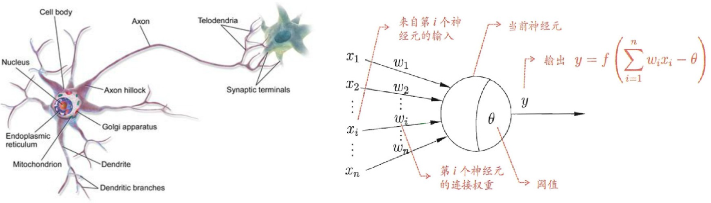

另外，我还整理总结了神经网络算法经典论文+示例代码，感兴趣的dd~

原文、姿.料 这儿~

一、先搞懂：神经网络像“多层计算器”

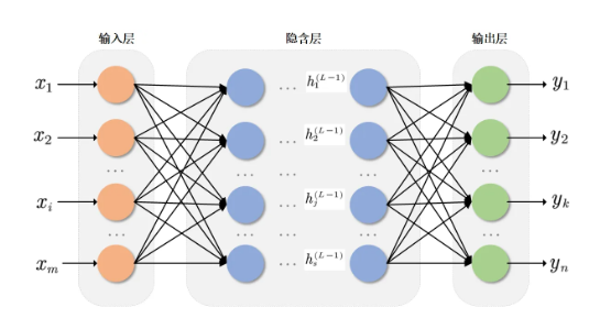
神经网络的核心是分层处理信息，就像工厂流水线：原料（输入数据）→加工（隐藏层）→成品（输出结果）。

1. 3大核心层（必记结构）

• 输入层：接收原始数据，比如识别图片时的像素值、预测房价时的面积/地段数据。
  ✅ 节点数=输入数据的维度（例：用2个特征预测房价，输入层就有2个节点）。
• 隐藏层：核心“加工间”，负责提取数据特征（比如从图片像素中识别“边缘”“颜色块”）。
  ✅ 层数和节点数可调整，简单任务1-2层足够，复杂任务（如图像识别）可能有几十层。
• 输出层：输出最终结果，比如“这张图是猫（1）还是狗（0）”“房价预测值150万”。
  ✅ 节点数=任务目标（二分类1个节点，多分类（如识别10种动物）10个节点）。

二、最小单元：神经元怎么“思考”？

每层的“节点”就是神经元，它的工作分3步，核心是加权计算+非线性转换。

1. 第一步：算“加权输入”（给输入打分）

每个输入会被赋予一个“权重”（$w_i$，可理解为“重要性”），再加上一个“偏置”（$b$，调整基准），求和得到净输入$z$。
公式：$z=w_1{x}_1+w_2{x}_2+...+w_n{x}_n+b={\sum }_{i=1}^n{w}_i{x}_i+b$

• $x_i$：神经元的第$i$个输入（比如输入层的“面积”“地段”）；
• $w_i$：对应$x_i$的权重（比如“面积”对房价影响大，$w$就大）；
• $b$：偏置项（避免输入全为0时神经元“不工作”）。

例子：用“面积（$x_1=100m^2$，$w_1=1.2$）”“地段（$x_2=8$分，$w_2=5$）”预测房价，偏置$b=20$，则：
$z=1.2\times 100+5\times 8+20=120+40+20=180$。

2. 第二步：过“激活函数”（加个“决策规则”）

净输入$z$是线性的，无法处理复杂问题（比如区分“猫”和“狗”的非线性特征），所以需要激活函数把$z$转换成非线性输出$a$。
常用3种激活函数（记这3个足够入门）：

激活函数	公式	作用	适用场景
Sigmoid	$a=\frac{1}{1+e^{-z}}$	把输出压到(0,1)之间，代表“概率”	二分类（如“是/否”“患病/健康”）
ReLU	$a=max(0,z)$	正数直接输出，负数输出0，解决“梯度消失”	隐藏层（最常用）
Tanh	$a=\frac{e^z-e^{-z}}{e^z+e^{-z}}$	把输出压到(-1,1)之间，均值更接近0	隐藏层（比Sigmoid收敛快）

接上面例子：若用ReLU激活，$a=max(0,180)=180$（可理解为房价的“初步预测值”）。

3. 第三步：输出结果（传给下一层或收尾）

激活后的$a$，要么作为下一层神经元的输入，要么作为最终结果（如输出层用Sigmoid输出“是猫的概率0.92”）。

三、核心流程：神经网络怎么“学”？（前向+反向）

神经网络的“学习”，本质是通过前向传播算预测值→反向传播调参数，不断降低“预测误差”。

1. 前向传播：从输入到输出的“正向计算”

简单说就是“逐层算输出”，把输入层数据通过权重、偏置、激活函数，一步步传到输出层，得到预测值$\hat{y}$。
以“输入层（2节点）→隐藏层（3节点）→输出层（1节点）”为例：

1. 输入层→隐藏层：每个隐藏节点用公式$z_{隐}=\sum w_{输入\to 隐}x+b_{隐}$算净输入，再过ReLU得$a_{隐}$；
2. 隐藏层→输出层：输出节点用$z_{输}=\sum w_{隐\to 输}{a}_{隐}+b_{输}$算净输入，再过Sigmoid得预测值$\hat{y}$。

2. 误差计算：先看“预测错多少”

有了预测值$\hat{y}$，需要和真实值$y$（比如标签“这是猫，$y=1$”）比，算“误差”。常用2种误差函数：

• 均方误差（MSE）：适用于回归任务（预测连续值，如房价、温度）
  公式：$Loss=\frac{1}{m}{\sum }_{i=1}^m({\hat{y}}_i-y_i{)}^2$
  （$m$是样本数，误差越大，Loss值越大）
• 交叉熵损失：适用于分类任务（预测离散类别，如猫/狗）
  公式（二分类）：$Loss=-\frac{1}{m}{\sum }_{i=1}^m[y_{i}log{\hat{y}}_i+(1-y_i)log(1-{\hat{y}}_i)]$

3. 反向传播：“倒着调参数”（最关键！）

误差出来后，要反过来调整所有的$w$（权重）和$b$（偏置），让下次预测更准。核心是用梯度下降找“最优参数”。

（1）核心逻辑：梯度下降

梯度是“误差对参数的导数”，代表“参数变化1单位时，误差的变化方向”。梯度下降的规则是：
参数 = 参数 - 学习率×梯度

• 学习率（$\eta$）：控制每次调整的“步长”，太大容易“跑过头”，太小收敛慢（常用0.01、0.1）；
• 梯度：若梯度为正，参数减“步长”→误差减小；若梯度为负，参数加“步长”→误差减小。

（2）具体步骤（简化版，小白能懂）

1. 算输出层误差：用误差函数对输出层的$z$求导，得到输出层误差${\delta }_{输}$；
2. 传误差到隐藏层：用输出层误差${\delta }_{输}$和权重$w_{隐\to 输}$，算隐藏层误差${\delta }_{隐}$（链式法则）；
3. 更参数：用误差$\delta$算梯度，再按“参数=参数-η×梯度”调整$w$和$b$。

假设某权重$w=2$，梯度=0.5，学习率$\eta =0.1$，则新权重：$w_{新}=2-0.1\times 0.5=1.95$。

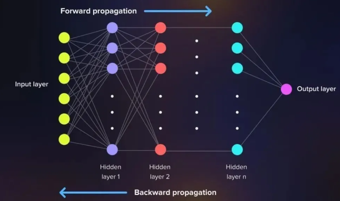
四、小白必知：2个实用知识点

1. 常见优化算法（比“普通梯度下降”更好用）

• SGD（随机梯度下降）：每次用1个样本更参数，快但波动大；
• Mini-Batch（小批量）：每次用10-100个样本更参数，平衡“速度”和“稳定”（最常用）；
• Adam：自带“动量”和“自适应学习率”，新手直接用，收敛快还不容易卡壳。

2. 简单代码示例（Python版，能跑通！）

用Python实现一个“预测房价”的简单神经网络（3层，输入2个特征，输出1个房价）：

import numpy as np
import matplotlib.pyplot as plt
from matplotlib.ticker import MaxNLocator
import os

# 创建保存图片的目录
if not os.path.exists('nn_plots'):
    os.makedirs('nn_plots')

# 1. 激活函数及其导数
def relu(z):
    return np.maximum(0, z)

def relu_derivative(z):
    return (z > 0).astype(float)  # ReLU derivative

def linear(z):
    return z  # Linear activation for output layer

def linear_derivative(z):
    return np.ones_like(z)  # Derivative of linear function is 1

# 2. 参数初始化 (使用Xavier初始化改进)
def init_params(input_dim, hidden_dim, output_dim):
    # Xavier initialization for more stable training
    w1 = np.random.randn(input_dim, hidden_dim) * np.sqrt(2 / (input_dim + hidden_dim))
    b1 = np.zeros((1, hidden_dim))  # Hidden layer bias
    
    w2 = np.random.randn(hidden_dim, output_dim) * np.sqrt(2 / (hidden_dim + output_dim))
    b2 = np.zeros((1, output_dim))  # Output layer bias
    
    return w1, b1, w2, b2

# 3. 前向传播
def forward(w1, b1, w2, b2, X):
    z1 = np.dot(X, w1) + b1  # Input to hidden layer net input
    a1 = relu(z1)            # Hidden layer output
    z2 = np.dot(a1, w2) + b2 # Hidden to output layer net input
    a2 = linear(z2)          # Output layer uses linear activation for regression
    
    return z1, a1, z2, a2

# 4. 损失计算 (MSE)
def compute_loss(a2, Y):
    m = Y.shape[0]
    loss = (1/(2*m)) * np.sum((a2 - Y)**2)
    return loss

def compute_loss_derivative(a2, Y):
    return (a2 - Y) / Y.shape[0]  # Derivative of MSE

# 5. 反向传播
def backward(w1, b1, w2, b2, z1, a1, z2, a2, X, Y):
    m = X.shape[0]
    
    # Output layer gradients
    dz2 = compute_loss_derivative(a2, Y) * linear_derivative(z2)
    dw2 = (1/m) * np.dot(a1.T, dz2)
    db2 = (1/m) * np.sum(dz2, axis=0, keepdims=True)
    
    # Hidden layer gradients
    dz1 = np.dot(dz2, w2.T) * relu_derivative(z1)
    dw1 = (1/m) * np.dot(X.T, dz1)
    db1 = (1/m) * np.sum(dz1, axis=0, keepdims=True)
    
    return dw1, db1, dw2, db2

# 6. 参数更新 (带学习率衰减)
def update_params(w1, b1, w2, b2, dw1, db1, dw2, db2, lr, decay_rate=0.0001, epoch=0):
    # Learning rate decay
    current_lr = lr / (1 + decay_rate * epoch)
    
    w1 = w1 - current_lr * dw1
    b1 = b1 - current_lr * db1
    w2 = w2 - current_lr * dw2
    b2 = b2 - current_lr * db2
    
    return w1, b1, w2, b2, current_lr

# 7. 可视化函数
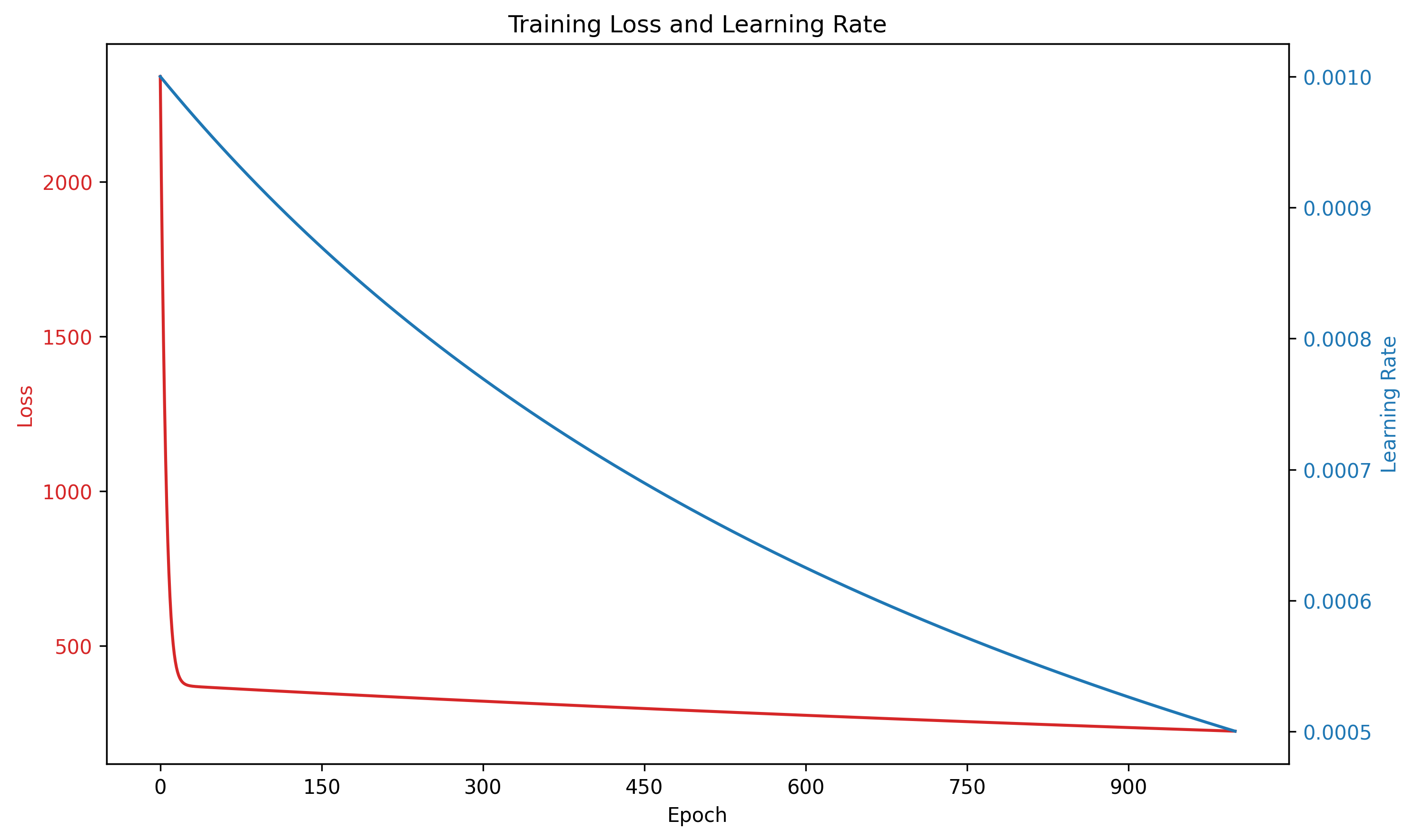
def plot_training_curve(losses, learning_rates, save_path='nn_plots/training_curve.png'):
    """Plot training loss and learning rate curves"""
    fig, ax1 = plt.subplots(figsize=(10, 6))
    
    color = 'tab:red'
    ax1.set_xlabel('Epoch')
    ax1.set_ylabel('Loss', color=color)
    ax1.plot(losses, color=color)
    ax1.tick_params(axis='y', labelcolor=color)
    ax1.xaxis.set_major_locator(MaxNLocator(integer=True))
    ax1.set_title('Training Loss and Learning Rate')
    
    ax2 = ax1.twinx()  # instantiate a second axes that shares the same x-axis
    color = 'tab:blue'
    ax2.set_ylabel('Learning Rate', color=color)  # we already handled the x-label with ax1
    ax2.plot(learning_rates, color=color)
    ax2.tick_params(axis='y', labelcolor=color)
    
    fig.tight_layout()  # otherwise the right y-label is slightly clipped
    plt.savefig(save_path, dpi=300, bbox_inches='tight')
    plt.close()

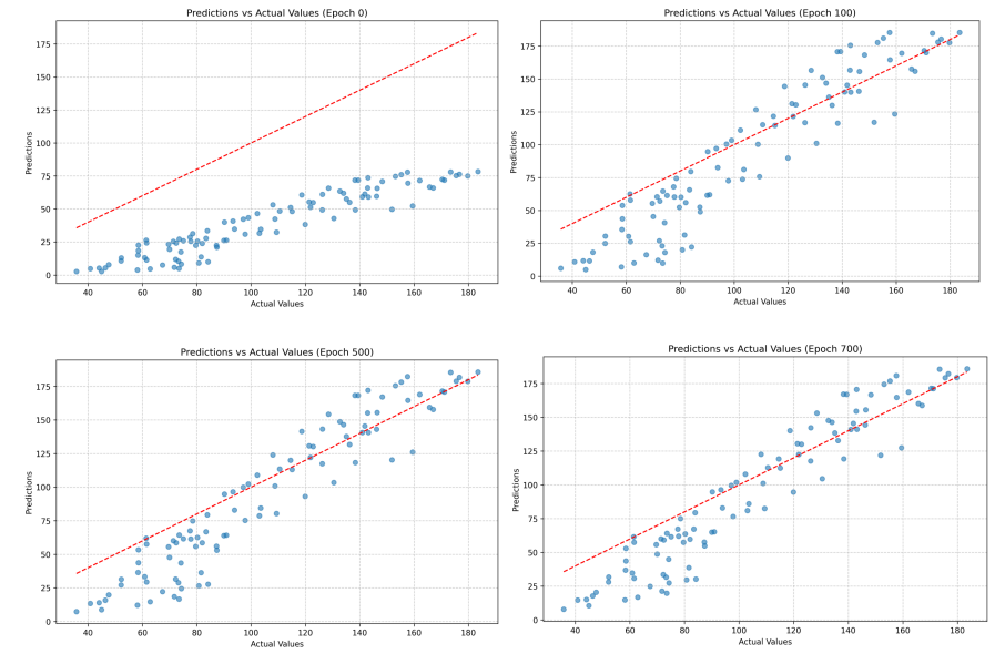
def plot_predictions_vs_actual(Y, predictions, epoch, save_dir='nn_plots/'):
    """Plot predictions vs actual values"""
    plt.figure(figsize=(10, 6))
    plt.scatter(Y, predictions, alpha=0.6)
    plt.plot([Y.min(), Y.max()], [Y.min(), Y.max()], 'r--')  # Perfect prediction line
    plt.xlabel('Actual Values')
    plt.ylabel('Predictions')
    plt.title(f'Predictions vs Actual Values (Epoch {epoch})')
    plt.grid(True, linestyle='--', alpha=0.7)
    plt.savefig(f'{save_dir}predictions_epoch_{epoch}.png', dpi=300, bbox_inches='tight')
    plt.close()

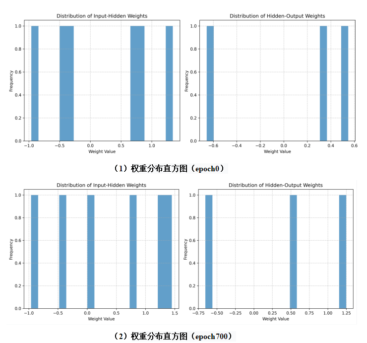
def plot_weight_distributions(w1, w2, epoch, save_dir='nn_plots/'):
    """Plot weight distributions"""
    fig, (ax1, ax2) = plt.subplots(1, 2, figsize=(12, 5))
    
    ax1.hist(w1.flatten(), bins=20, alpha=0.7)
    ax1.set_title('Distribution of Input-Hidden Weights')
    ax1.set_xlabel('Weight Value')
    ax1.set_ylabel('Frequency')
    ax1.grid(True, linestyle='--', alpha=0.7)
    
    ax2.hist(w2.flatten(), bins=20, alpha=0.7)
    ax2.set_title('Distribution of Hidden-Output Weights')
    ax2.set_xlabel('Weight Value')
    ax2.set_ylabel('Frequency')
    ax2.grid(True, linestyle='--', alpha=0.7)
    
    plt.tight_layout()
    plt.savefig(f'{save_dir}weights_dist_epoch_{epoch}.png', dpi=300, bbox_inches='tight')
    plt.close()

# 8. 主训练函数
def train_model(X, Y, input_dim, hidden_dim, output_dim, epochs=1000, lr=0.1, decay_rate=0.0001):
    # Initialize parameters
    w1, b1, w2, b2 = init_params(input_dim, hidden_dim, output_dim)
    
    # Lists to track training progress
    losses = []
    learning_rates = []
    
    # Initial predictions
    _, _, _, initial_preds = forward(w1, b1, w2, b2, X)
    plot_predictions_vs_actual(Y, initial_preds, 0)
    plot_weight_distributions(w1, w2, 0)
    
    # Training loop
    for epoch in range(epochs):
        # Forward propagation
        z1, a1, z2, a2 = forward(w1, b1, w2, b2, X)
        
        # Compute loss
        loss = compute_loss(a2, Y)
        losses.append(loss)
        
        # Backward propagation
        dw1, db1, dw2, db2 = backward(w1, b1, w2, b2, z1, a1, z2, a2, X, Y)
        
        # Update parameters with learning rate decay
        w1, b1, w2, b2, current_lr = update_params(
            w1, b1, w2, b2, dw1, db1, dw2, db2, lr, decay_rate, epoch
        )
        learning_rates.append(current_lr)
        
        # Print progress and save plots at intervals
        if epoch % 100 == 0:
            print(f"Epoch {epoch}, Loss: {loss:.4f}, Learning Rate: {current_lr:.6f}")
            
            # Save predictions plot at certain epochs
            if epoch in [100, 300, 500, 700, epochs-1]:
                plot_predictions_vs_actual(Y, a2, epoch)
                plot_weight_distributions(w1, w2, epoch)
    
    # Final plots
    plot_training_curve(losses, learning_rates)
    
    return w1, b1, w2, b2, losses

# 9. 测试模型
if __name__ == "__main__":
    # Generate synthetic data (house prices based on area and location)
    np.random.seed(42)  # For reproducibility
    num_samples = 100
    
    # Features: area (in 100 sq.m), location score (1-10)
    X = np.random.rand(num_samples, 2)
    X[:, 0] = X[:, 0] * 100  # Area: 0-100 sq.m
    X[:, 1] = X[:, 1] * 9 + 1  # Location score: 1-10
    
    # True price function with some noise
    true_weights = np.array([1.2, 5.0])  # Weights for area and location
    true_bias = 20.0  # Base price
    noise = np.random.normal(0, 5, (num_samples, 1))  # Add some noise
    Y = (X @ true_weights).reshape(-1, 1) + true_bias + noise
    
    # Train the model
    print("Starting model training...")
    w1, b1, w2, b2, losses = train_model(
        X, Y, 
        input_dim=2, 
        hidden_dim=3, 
        output_dim=1, 
        epochs=1000, 
        lr=0.001,  # Lower learning rate for more stable training
        decay_rate=0.001
    )
    
    # Final evaluation
    _, _, _, final_preds = forward(w1, b1, w2, b2, X)
    final_loss = compute_loss(final_preds, Y)
    print(f"\nFinal training loss: {final_loss:.4f}")
    
    # Print true vs learned parameters for comparison
    print("\nTrue weights:", true_weights)
    print("True bias:", true_bias)
    
    # Print model architecture summary
    print("\nModel Architecture:")
    print(f"Input layer: {X.shape[1]} features")
    print(f"Hidden layer: {w1.shape[1]} neurons")
    print(f"Output layer: {w2.shape[1]} output")

五、总结：小白入门3个关键

1. 结构：输入→隐藏→输出，每层靠神经元（加权+激活）处理；
2. 流程：前向算预测→误差算对错→反向调参数（梯度下降）；
3. 工具：不用死磕数学，先跑通简单代码（比如上面的Python示例），再慢慢理解细节。

神经网络没那么玄乎，入门先抓“分层”“加权”“梯度下降”这3个核心，后续再学CNN（图像）、RNN（文本）就顺理成章啦！