# Importing libraries
import tensorflow as tf
import numpy as np
import os
import random
import pandas as pd
import seaborn as sns
from datetime import datetime
import matplotlib.pyplot as plt
plt.rc('font', size=16)
from sklearn.preprocessing import MinMaxScaler
import warnings
warnings.filterwarnings('ignore')
tf.get_logger().setLevel('ERROR')


tfk = tf.keras
tfkl = tf.keras.layers


# Random seed for reproducibility
seed = 42
random.seed(seed)
os.environ['PYTHONHASHSEED'] = str(seed)
np.random.seed(seed)
tf.random.set_seed(seed)
tf.compat.v1.set_random_seed(seed)
# Plotting the head of the dataset
dataset = pd.read_csv('../input/an2dl-homework-2/Training.csv')
print(dataset.shape)
dataset.head()
(68528, 7)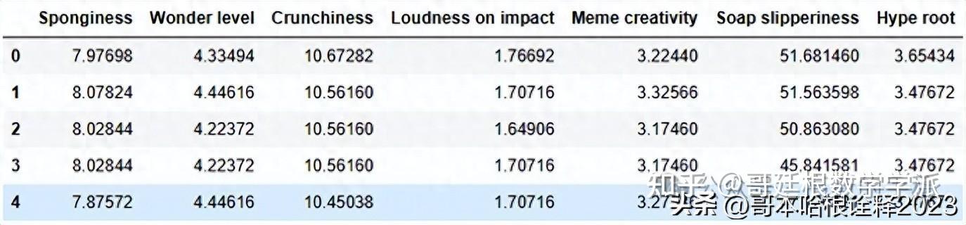

dataset.info()
<class 'pandas.core.frame.DataFrame'>
RangeIndex: 68528 entries, 0 to 68527
Data columns (total 7 columns):
 #   Column              Non-Null Count  Dtype  
---  ------              --------------  -----  
 0   Sponginess          68528 non-null  float64
 1   Wonder level        68528 non-null  float64
 2   Crunchiness         68528 non-null  float64
 3   Loudness on impact  68528 non-null  float64
 4   Meme creativity     68528 non-null  float64
 5   Soap slipperiness   68528 non-null  float64
 6   Hype root           68528 non-null  float64
dtypes: float64(7)
memory usage: 3.7 MB
def inspect_dataframe(df, columns):
    figs, axs = plt.subplots(len(columns), 1, sharex=True, figsize=(17,17))
    for i, col in enumerate(columns):
        axs[i].plot(df[col])
        axs[i].set_title(col)
    plt.show()


# Plotting time series
inspect_dataframe(dataset, dataset.columns)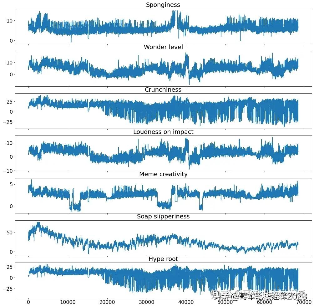

# Setting window, stringe, validation size and telescope
window = 300
stride = 10
validation_size = 13700
target_labels = dataset.columns
telescope = 864
X_train_raw = dataset.iloc[:-validation_size]
X_validation_raw = dataset.iloc[-validation_size:]


print(X_train_raw.shape, X_validation_raw.shape)


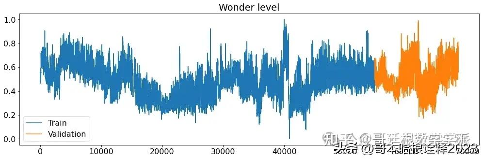
# Normalize both features and labels
X_min = X_train_raw.min()
X_max = X_train_raw.max()


X_train_raw = (X_train_raw-X_min)/(X_max-X_min)
X_validation_raw = (X_validation_raw-X_min)/(X_max-X_min)
(54828, 7) (13700, 7)
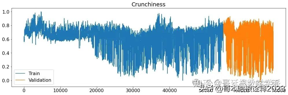
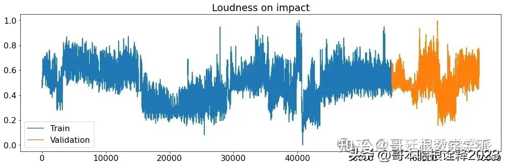
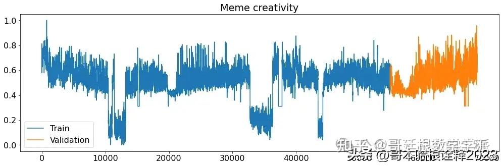
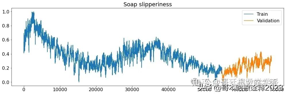
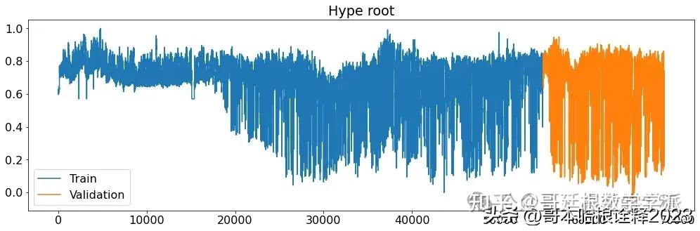
def printplots():
    for i in range(X_train_raw.shape[1]):
        plt.figure(figsize=(17,5))
        plt.plot(X_train_raw[(target_labels[i])], label='Train')
        plt.plot(X_validation_raw[(target_labels[i])], label='Validation')
        plt.title((target_labels[i]))
        plt.legend()
        plt.show()
# Normalized time series
printplots()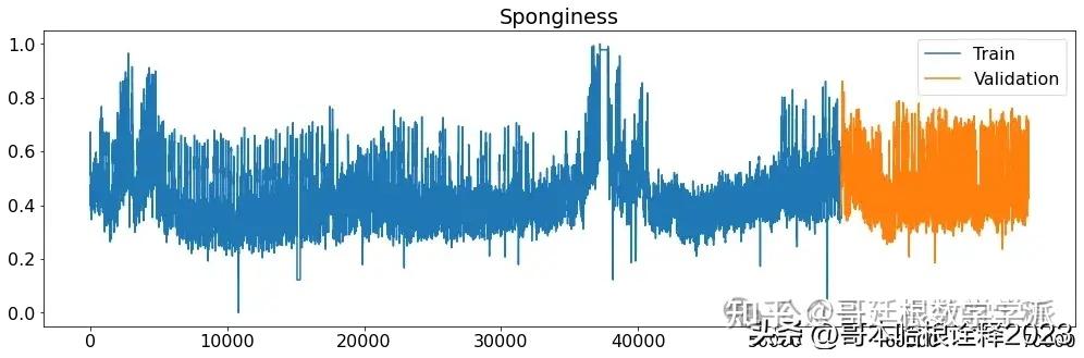

future = dataset[-window:]
future = (future-X_min)/(X_max-X_min)
future = np.expand_dims(future, axis=0)
future.shape
(1, 300, 7)
def build_sequences(df, target_labels=target_labels, window=window, stride=20, telescope=100):
    
    assert window % stride == 0
    dataset = []
    labels = []
    temp_df = df.copy().values
    temp_label = df[target_labels].copy().values
    padding_len = len(df)%window


    if(padding_len != 0):
        # Compute padding length
        padding_len = window - len(df)%window
        padding = np.zeros((padding_len,temp_df.shape[1]), dtype='float64')
        temp_df = np.concatenate((padding,df))
        padding = np.zeros((padding_len,temp_label.shape[1]), dtype='float64')
        temp_label = np.concatenate((padding,temp_label))
        assert len(temp_df) % window == 0


    for idx in np.arange(0,len(temp_df)-window-telescope,stride):
        dataset.append(temp_df[idx:idx+window])
        labels.append(temp_label[idx+window:idx+window+telescope])


    dataset = np.array(dataset)
    labels = np.array(labels)
    return dataset, labels
X_train, y_train = build_sequences(X_train_raw, target_labels, window, stride, telescope)
X_val, y_val = build_sequences(X_validation_raw, target_labels, window, stride, telescope)
X_train.shape, y_train.shape, X_val.shape, y_val.shape
((5374, 300, 7), (5374, 864, 7), (1264, 300, 7), (1264, 864, 7))
input_shape = X_train.shape[1:]
output_shape = y_train.shape[1:]
batch_size = 32
epochs = 200
# Model of the exercise session


def build_CONV_LSTM_model(input_shape, output_shape):
    
    input_layer = tfkl.Input(shape=input_shape, name='Input')


    convlstm = tfkl.Bidirectional(tfkl.LSTM(64, return_sequences=True, recurrent_dropout=0.2))(input_layer)
    convlstm = tfkl.Conv1D(128, 3, padding='same', activation='relu')(convlstm)
    convlstm = tfkl.MaxPool1D()(convlstm)
    convlstm = tfkl.Bidirectional(tfkl.LSTM(128, return_sequences=True, recurrent_dropout=0.2))(convlstm)
    convlstm = tfkl.Conv1D(256, 3, padding='same', activation='relu')(convlstm)
    convlstm = tfkl.GlobalAveragePooling1D()(convlstm)
    convlstm = tfkl.Dropout(.5)(convlstm)


    dense = tfkl.Dense(output_shape[-1]*output_shape[-2], activation='relu')(convlstm)
    output_layer = tfkl.Reshape((output_shape[-2],output_shape[-1]))(dense)
    output_layer = tfkl.Conv1D(output_shape[-1], 1, padding='same')(output_layer)


    # Connect input and output through the Model class
    model = tfk.Model(inputs=input_layer, outputs=output_layer, name='model')


    # Compile the model
    model.compile(loss=tfk.losses.MeanSquaredError(), optimizer=tfk.optimizers.Adam(), metrics=[tfk.metrics.RootMeanSquaredError()])


    # Return the model
    return model
model = build_CONV_LSTM_model(input_shape, output_shape)
model.summary()
Model: "model"
_________________________________________________________________
Layer (type)                 Output Shape              Param #   
=================================================================
Input (InputLayer)           [(None, 300, 7)]          0         
_________________________________________________________________
bidirectional (Bidirectional (None, 300, 128)          36864     
_________________________________________________________________
conv1d (Conv1D)              (None, 300, 128)          49280     
_________________________________________________________________
max_pooling1d (MaxPooling1D) (None, 150, 128)          0         
_________________________________________________________________
bidirectional_1 (Bidirection (None, 150, 256)          263168    
_________________________________________________________________
conv1d_1 (Conv1D)            (None, 150, 256)          196864    
_________________________________________________________________
global_average_pooling1d (Gl (None, 256)               0         
_________________________________________________________________
dropout (Dropout)            (None, 256)               0         
_________________________________________________________________
dense (Dense)                (None, 6048)              1554336   
_________________________________________________________________
reshape (Reshape)            (None, 864, 7)            0         
_________________________________________________________________
conv1d_2 (Conv1D)            (None, 864, 7)            56        
=================================================================
Total params: 2,100,568
Trainable params: 2,100,568
Non-trainable params: 0
_________________________________________________________________
# Training
history = model.fit(
    x = X_train,
    y = y_train,
    batch_size = batch_size,
    epochs = epochs,
    validation_data = (X_val,y_val),
    callbacks = [tfk.callbacks.EarlyStopping(monitor='val_loss', mode='min', patience=10, restore_best_weights=True),
                tfk.callbacks.ReduceLROnPlateau(monitor='val_loss', mode='min', patience=5, factor=0.5, min_lr=1e-5)]
).history
best_epoch = np.argmin(history['val_loss'])
plt.figure(figsize=(17,4))
plt.plot(history['loss'], label='Training loss', alpha=.8, color='#ff7f0e')
plt.plot(history['val_loss'], label='Validation loss', alpha=.9, color='#5a9aa5')
plt.axvline(x=best_epoch, label='Best epoch', alpha=.3, ls='--', color='#5a9aa5')
plt.title('Root Mean Squared Error (Loss)')
plt.legend()
plt.grid(alpha=.3)
plt.show()


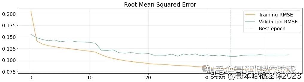
plt.figure(figsize=(17,4))
plt.plot(history['root_mean_squared_error'], label='Training RMSE', alpha=.8, color='#ff7f0e')
plt.plot(history['val_root_mean_squared_error'], label='Validation RMSE', alpha=.9, color='#5a9aa5')
plt.axvline(x=best_epoch, label='Best epoch', alpha=.3, ls='--', color='#5a9aa5')
plt.title('Root Mean Squared Error')
plt.legend()
plt.grid(alpha=.3)
plt.show()


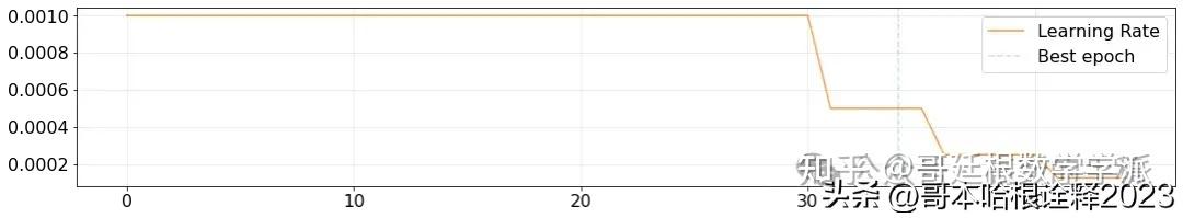
plt.figure(figsize=(18,3))
plt.plot(history['lr'], label='Learning Rate', alpha=.8, color='#ff7f0e')
plt.axvline(x=best_epoch, label='Best epoch', alpha=.3, ls='--', color='#5a9aa5')
plt.legend()
plt.grid(alpha=.3)
plt.show()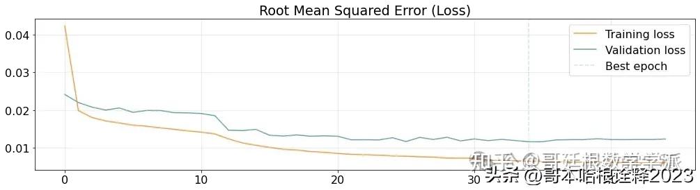

model.save('TS_Direct')
# Predict the test set 
predictions = model.predict(X_val)
print(predictions.shape)


mean_squared_error = tfk.metrics.mse(y_val.flatten(),predictions.flatten())
mean_absolute_error = tfk.metrics.mae(y_val.flatten(),predictions.flatten())
mean_squared_error, mean_absolute_error
(1264, 864, 7)
def inspect_multivariate_prediction(X, y, pred, columns, telescope, idx=None):
    if(idx==None):
        idx=np.random.randint(0,len(X))


    figs, axs = plt.subplots(len(columns), 1, sharex=True, figsize=(17,17))
    for i, col in enumerate(columns):
        axs[i].plot(np.arange(len(X[0,:,i])), X[idx,:,i])
        axs[i].plot(np.arange(len(X[0,:,i]), len(X_train[0,:,i])+telescope), y[idx,:,i], color='orange')
        axs[i].plot(np.arange(len(X[0,:,i]), len(X_train[0,:,i])+telescope), pred[idx,:,i], color='green')
        axs[i].set_title(col)
        axs[i].set_ylim(0,1)
    plt.show()
inspect_multivariate_prediction(X_val, y_val, predictions, target_labels, telescope)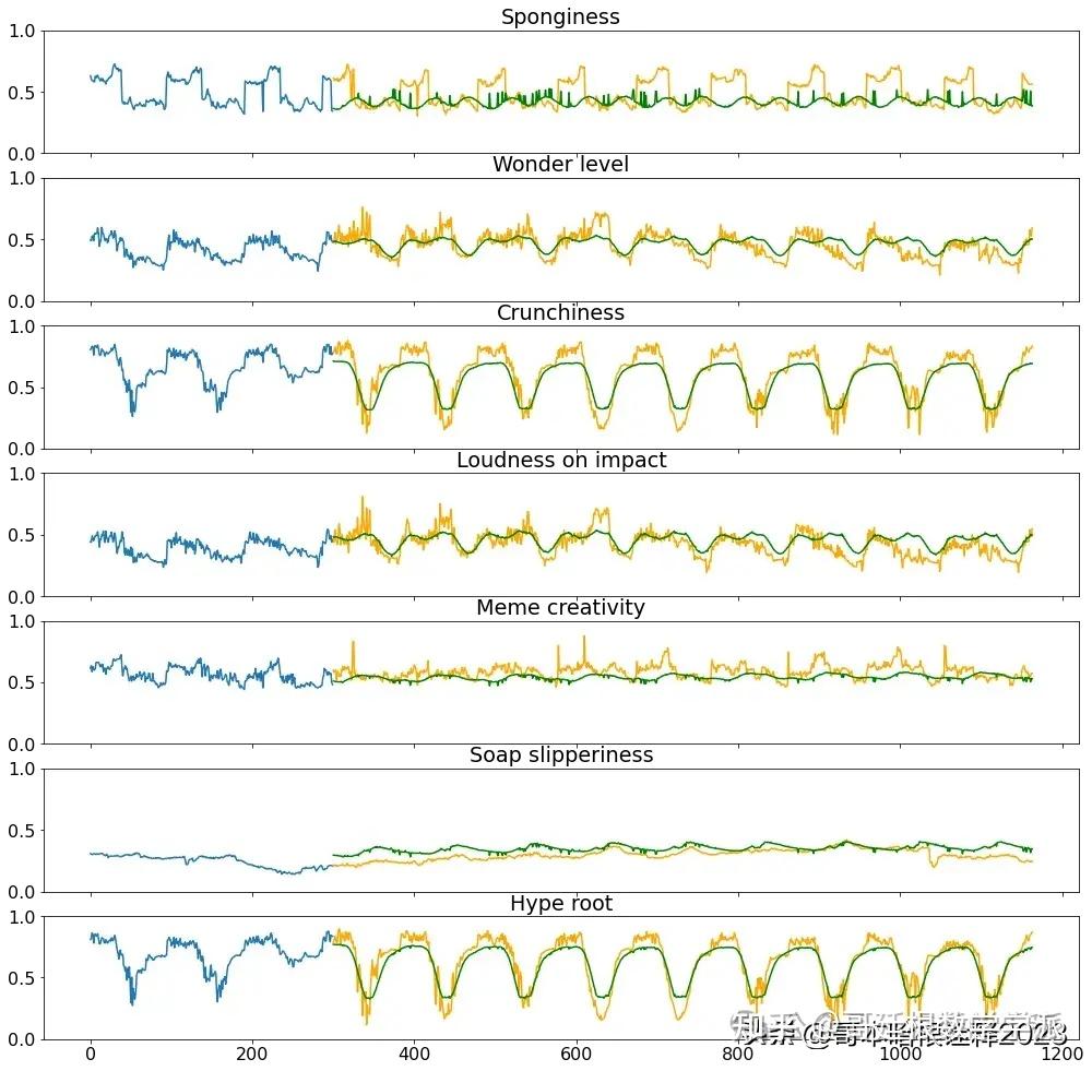

学术咨询

担任《Mechanical System and Signal Processing》《中国电机工程学报》等期刊审稿专家，擅长领域：信号滤波/降噪，机器学习/深度学习，时间序列预分析/预测，设备故障诊断/缺陷检测/异常检测。

分割线分割线分割线分割线分割线分割线分割线分割线分割线

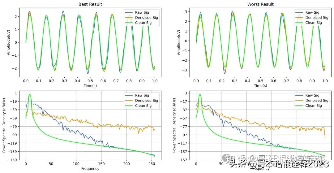
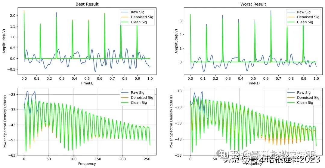
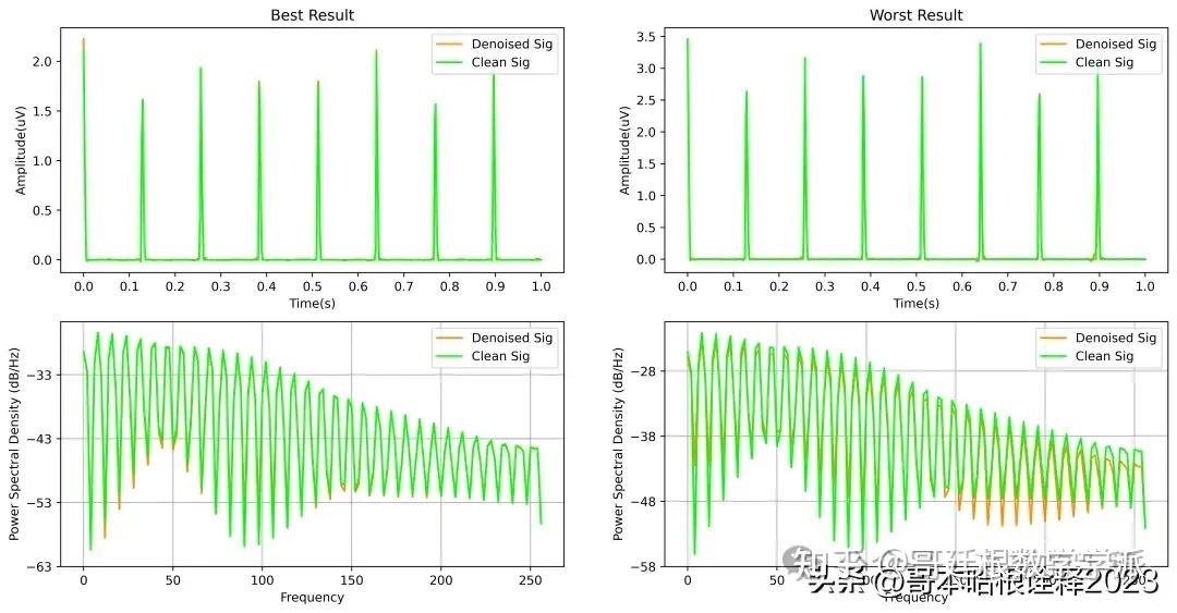
基于深度学习的超低频信号降噪方法（Python，ipynb文件）

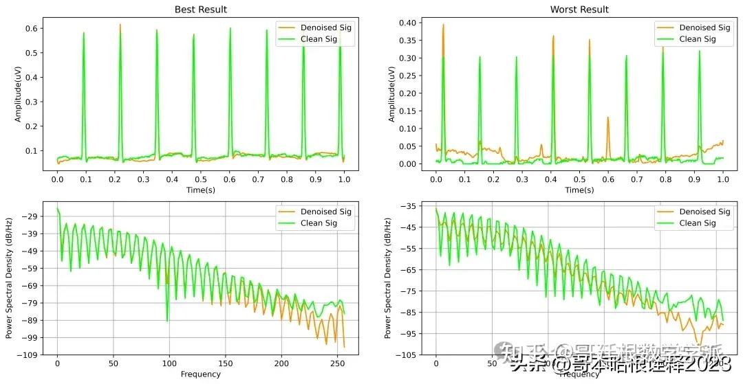
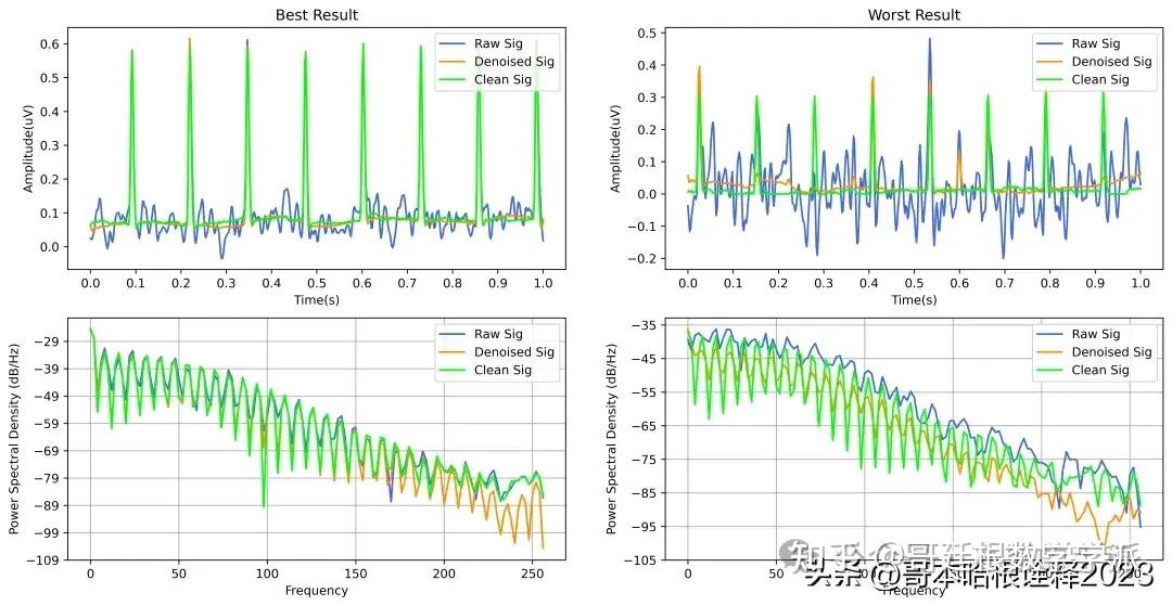
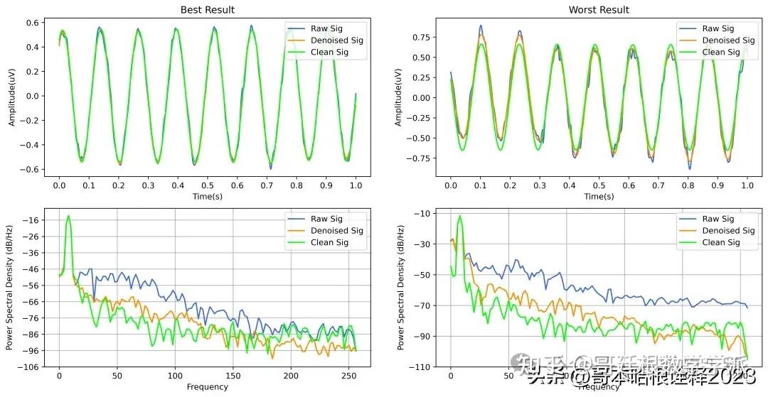
完整代码通过学术咨询获得