我们采用 python tensorflow1.14 来处理多分类问题.

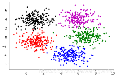
给定一个数据集，并对其可视化有

import tensorflow as tf
import numpy as np
import matplotlib.pyplot as plt
import time


# set seed

np.random.seed(1234)
tf.set_random_seed(1234)


# data set

sigma = np.array([[1,0],[0,1]])
mu1 = np.array([1, -1])
x1 = np.random.multivariate_normal(mu1, sigma, 200)
mu2 = np.array([5, -4])
x2 = np.random.multivariate_normal(mu2, sigma, 200)
mu3 = [1,4]
x3 = np.random.multivariate_normal(mu3, sigma, 200)
mu4 = np.array([6,4])
x4 = np.random.multivariate_normal(mu4, sigma, 200)
mu5 = np.array([7,0])
x5 = np.random.multivariate_normal(mu5, sigma, 200)


# show the data 

plt.plot(x1[:, 0],x1[:, 1],'r.')
plt.plot(x2[:, 0],x2[:, 1],'b.')
plt.plot(x3[:, 0],x3[:, 1],'k.')
plt.plot(x4[:, 0],x4[:, 1],'m.')
plt.plot(x5[:, 0],x5[:, 1],'g.')

我们把数据分为训练集和测试集（6:4），并且将数据标签转化为 one-hot 编码，即

# Separate the data set : training data and test data 

index1 = np.random.choice(200, 200, replace=False)
index2 = np.random.choice(200, 200, replace=False)
index3 = np.random.choice(200, 200, replace=False)
index4 = np.random.choice(200, 200, replace=False)
index5 = np.random.choice(200, 200, replace=False)

x1_train = x1[index1[0:120], :]
x2_train = x2[index1[0:120], :]
x3_train = x3[index1[0:120], :]
x4_train = x4[index1[0:120], :]
x5_train = x5[index1[0:120], :]

x1_test = x1[index1[120:], :]
x2_test = x2[index1[120:], :]
x3_test = x3[index1[120:], :]
x4_test = x4[index1[120:], :]
x5_test = x5[index1[120:], :]

X_train = np.vstack((x1_train, x2_train, x3_train, x4_train, x5_train))
X_test = np.vstack((x1_test, x2_test, x3_test, x4_test, x5_test))
train_label = np.matrix([[1, 0, 0, 0, 0]] * 120 + [[0, 1, 0, 0, 0]] * 120 + \
                        [[0, 0, 1, 0, 0]] * 120 + [[0, 0, 0, 1, 0]] * 120 +\
                            [[0, 0, 0, 0, 1]] * 120)
test_label = np.matrix([[1, 0, 0, 0, 0]] * 80 + [[0, 1, 0, 0, 0]] * 80 + \
                        [[0, 0, 1, 0, 0]] * 80 + [[0, 0, 0, 1, 0]] * 80 +\
                            [[0, 0, 0, 0, 1]] * 80)

我们采用三层前向神经网络来优化这个任务, 其中每层的神经元个数取20, 初始化取 xavier initialization,优化处理器取 GradientDescentOptimizer, 学习率取 0.001, 激活函数选取 sigmoid 函数, 迭代次数为 1000.

N = 20
layers = [2, N, N, N, 5]
nIter = 100

# define neural network structure

#tf.palceholder 
x_tf=tf.placeholder(tf.float32,shape=[None,X_train.shape[1]])
y_tf=tf.placeholder(tf.float32,shape=[None,train_label.shape[1]])
def initialize_NN(layers):        
    weights = []
    biases = []
    num_layers = len(layers) 
    for l in range(0,num_layers-1):
        W = xavier_init(size=[layers[l], layers[l+1]])
        b = tf.Variable(tf.zeros([1,layers[l+1]], dtype=tf.float32), dtype=tf.float32)
        weights.append(W)
        biases.append(b)        
    return weights, biases
    
def xavier_init(size):
    in_dim = size[0]
    out_dim = size[1]        
    xavier_stddev = np.sqrt(2/(in_dim + out_dim))
    return tf.Variable(tf.truncated_normal([in_dim, out_dim], stddev=xavier_stddev), dtype=tf.float32)

def neural_net(X, weights, biases):
    num_layers = len(weights) + 1
    H = X
    for l in range(0,num_layers-2):
        W = weights[l]
        b = biases[l]
        H = tf.sigmoid(tf.add(tf.matmul(H, W), b))
    W = weights[-1]
    b = biases[-1]
    Y = tf.add(tf.matmul(H, W), b)
    return Y

in_weights, in_biases = initialize_NN(layers)

def net(X):
    h = neural_net(X, in_weights, in_biases)
    return h
output = net(x_tf)

#loss
y_model = tf.nn.softmax(output)
loss = -tf.reduce_sum(y_tf * tf.log(y_model))
correct_prediction = tf.equal(tf.argmax(y_model, 1), tf.argmax(y_tf, 1))
accuracy = tf.reduce_mean(tf.cast(correct_prediction, "float")) 

# Optimization

optimizer_GradientDescent = tf.train.GradientDescentOptimizer(0.001)
train_op_Adam =optimizer_GradientDescent.minimize(loss)

 训练模型

# tf session

sess = tf.Session()
init = tf.global_variables_initializer()
sess.run(init)

tf_dict = {x_tf:X_train, y_tf:train_label}
start_time = time.time()
for it in range(nIter):
    sess.run(train_op_Adam, tf_dict)
        
    # Print
    if it % 100 == 0:
        elapsed = time.time() - start_time
        loss_value =sess.run(loss, tf_dict)
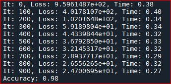
        print('It: %d, Loss: %.7e, Time: %.2f' % 
              (it, loss_value, elapsed))
        start_time = time.time()

测试其在测试集上的正确率

accuracy = sess.run(accuracy, feed_dict={x_tf:X_test,y_tf:test_label})
print("Accuracy: %.2f" % accuracy)

 得到精度为

 至此，便完成了多分类问题。