介绍 (Introduction)

In any company, there is an embedded desire to predict its future revenue and future sales. The basic recipe is:

在任何公司中，都存在着预测其未来收入和未来销售额的内在愿望。 基本配方是：

Collect historical data related to previous sales and use it to predict expected sales.

收集与以前的销售有关的历史数据，并用它来预测预期的销售。

Over the last ten years, the rise of deep learning as the driving force behind all imaginable machine learning benchmarks revolutionized the field: be it in computer vision, language and so many others. Recently, one could argue that deep learning has restructured the potential future of sales forecasting by allowing models to encode for multiple time series in a single model as well as account for categorical variables. My goal today is:

在过去的十年中，深度学习的兴起成为所有可想象的机器学习基准背后的推动力，彻底改变了该领域：无论是在计算机视觉，语言还是许多其他领域。 最近，有人可能会争辩说，深度学习通过允许模型对单个模型中的多个时间序列进行编码并考虑分类变量，从而重构了销售预测的潜在未来。 我今天的目标是：

To walk you through the basic intuitions behind the main concepts and models for sales forecasting from a time-series perspective and discuss what kind of capabilities recent deep learning models could bring to the table.

从时间序列的角度向您介绍销售预测的主要概念和模型背后的基本直觉，并讨论最近的深度学习模型可以带来哪些功能。

阅读建议 (Reading Suggestions)

In case you feel like you need to brush up on the basics of sales forecasting and time-series, I recommend these 3 reads:

如果您觉得需要重新了解销售预测和时间序列的基础知识，我建议您阅读以下三篇文章：

• Harvard business article on the fundamentals of sales forecasting.

  哈佛商业文章中有关销售预测的基础知识。

• TDS article by @Marco Peixeiro from on @Towards Data Science (really comprehensive and instructive).

  @Marco Peixeiro在@Towards Data Science上发表的TDS文章 (非常全面且具有指导意义)。

• “Time Series Forecasting Principles with Amazon Forecast”. They do a thorough job of explaining how Sales Forecasting works, as well as what are the challenges and problems one might encounter in the field.

  “使用Amazon Forecast进行时间序列预测的原理” 。 他们做了详尽的工作，解释了“销售预测”的工作原理以及该领域可能遇到的挑战和问题。

销售预测问题 (The Sales Forecasting Problem)

Sales forecasting is all about using historical data to inform decision making.

销售预测是关于使用历史数据来指导决策的全部。

A simple forecasting cycle looks like this:

一个简单的预测周期如下所示：

On its core, this is a time series problem: given some data in time, we want to predict the dynamics of that same data in the future. To do this, we require some trainable model of these dynamics.

从根本上讲，这是一个时间序列问题：给定一些及时的数据，我们希望将来预测相同数据的动态。 为此，我们需要一些动态的可训练模型。

According to Amazon’s time series forecasting principles, forecasting is a hard problem for 2 reasons:

根据Amazon的时间序列预测原则 ，由于以下两个原因，预测是一个难题：

• Incorporating large volumes of historical data, which can lead to missing important information about the past of the target data dynamics.
  合并大量历史数据可能会导致丢失有关目标数据动态变化的过去的重要信息。
• Incorporating related yet independent data (holidays/events, locations, marketing promotions)
  整合相关但独立的数据(节假日/活动，位置，营销促销)

Besides these, one of the central aspects of sales forecasting is that accuracy is key:

除此之外，销售预测的主要方面之一是准确性是关键：

• If the forecast is too high it may lead to over-investing and therefore losing money.
  如果预测值太高，则可能导致过度投资，从而造成资金损失。
• If the forecast is too low it may lead to under-investing and therefore losing opportunity.
  如果预测值太低，则可能导致投资不足，从而失去机会。

Incorporating exogenous factors like the weather, time and spatial location could be beneficial for a prediction. In this medium piece by Liudmyla Taranenko, she mentions a great example discussing how on-demand ride services like UBER, Lyft or Didi Chuxing must take into account factors like weather conditions (like humidity and temperature), time of the day or day of the week to do its demand forecasting. Therefore, good forecasting models should have mechanisms that enable them to account for such factors.

结合天气，时间和空间位置等外在因素可能有助于预测。 在这种媒介片由Liudmyla Taranenko ，她提到了一个很好的例子，讨论如何点播喜欢UBER，Lyft或迪迪楚星程服务，必须考虑多种因素，如天气条件(如温度和湿度)的一天或一天的时间一周进行需求预测。 因此，良好的预测模型应具有使它们能够考虑这些因素的机制。

In sum, what do we know so far?

总而言之，到目前为止我们知道什么？

• We know that forecasting is a hard problem where accuracy really matters.
  我们知道，预测是一个很难解决的问题，其中准确性至关重要。
• We know that there are exogenous factors that come into play that are hard to account for.
  我们知道，有些外在因素在起作用，很难解释。

What we don’t know yet is:

我们还不知道的是：

• What are the traditional forecasting methods and why they might succumb to these challenges.
  传统的预测方法是什么，为什么它们会屈服于这些挑战。
• How is it that deep learning methods could help, and what are some of the prospects to replace traditional models.
  深度学习方法将如何提供帮助，以及替代传统模型的前景如何？

预测模型的类型 (Types of Forecasting Models)

According to this article featured in the Harvard business review, there are three types of Forecasting techniques:

根据《哈佛商业评论》上的这篇文章 ，有三种类型的预测技术：

• Qualitative techniques: usually involve expert opinion or information about special events.

  定性技术 ：通常涉及专家意见或有关特殊事件的信息。

• Time series analysis and projection: involve historical data, finding structure in the dynamics of the data like cyclical patterns, trends and growth rates.

  时间序列分析和预测 ：涉及历史数据，在数据动态中寻找结构，例如周期性变化，趋势和增长率。

• Causal models: these models involve the relevant causal relationships that may include pipeline considerations like inventories or market survey information. They can incorporate the results of a time series analysis.

  因果模型 ：这些模型涉及相关的因果关系，其中可能包括管道方面的考虑，例如库存或市场调查信息。 他们可以合并时间序列分析的结果。

We will focus on the time series analysis approach which has been the driving force behind traditional forecasting methods and it can give a comprehensive layout of the forecasting landscape.

我们将重点关注时间序列分析方法，该方法一直是传统预测方法的推动力，并且可以对预测格局进行全面布局。

时间序列方法 (Time Series Approach)

A time series is a sequence of data points taken at successive, equally-spaced points in time that can be used to predict the future. A time series analysis model involves using historical data to forecast the future. It looks in the dataset for features such as trends, cyclical fluctuations, seasonality, and behavioral patterns.

时间序列是在连续的等间隔时间点获取的数据点序列，可用于预测未来。 时间序列分析模型涉及使用历史数据来预测未来。 它在数据集中查找诸如趋势，周期性波动，季节性和行为模式等特征。

The three key general ideas that are fundamental to consider, when dealing with a sales forecasting problem tackled from a time series perspective, are:

在处理从时间序列角度解决的销售预测问题时，需要考虑的三个基本基本概念是：

• Repeating patterns
  重复图案
• Static patterns
  静态模式
• Trends
  发展趋势

Now we’ll look into each of these factors and write code that will allow us to understand them intuitively. After that, we will see what modern deep learning models could bring to the table.

现在，我们将研究所有这些因素，并编写使我们能够直观地理解它们的代码。 之后，我们将看到现代深度学习模型可以带来什么。

重复图案 (Repeating Patterns)

When looking at a time series data, one element that we are looking for is a pattern that repeats in time. One key concept related to this idea is autocorrelation.

当查看时间序列数据时，我们要寻找的一个元素是时间重复的模式。 与这个想法有关的一个关键概念是自相关 。

Intuitively, autocorrelation corresponds to the similarity between observations as a function of the time lag between them.

直觉上， 自相关与观察之间的相似性相对应，这取决于它们之间的时间滞后。

What does that mean? It refers to the idea of finding structure on the dynamics of the observations in a time-series by looking at the correlation between observations with themselves (i.e. “auto”) at different time points. It is one of the main tools for finding repeating patterns.

那是什么意思？ 它指的是通过观察不同时间点的观察值与自身之间的相关性(即“自动”)来发现时间序列中的动力学结构的想法。 它是查找重复模式的主要工具之一。

To clarify this, let’s take a look at the publicly available weather dataset from kaggle and plot both its raw temperature data as well as an autocorrelation graph.

为了澄清这一点，让我们看一下kaggle上公开可用的天气数据集，并绘制其原始温度数据和自相关图。

The steps will be:

步骤将是：

• Load our dataset
  加载我们的数据集
• Clean the dates column
  清理日期列
• Plot raw weather data
  绘制原始天气数据

• Plot an autocorrelation plot using statsmodels

  使用statsmodels绘制自相关图

import pandas as pd
import matplotlib.pyplot as plt
import seaborn as sns
sns.set()
from statsmodels.graphics.tsaplots import plot_acf
green = sns.color_palette("deep", 8)[2]
blue = sns.color_palette("deep", 8)[0]
# Loading the dataset
df_weather = pd.read_csv("data/weatherHistory.csv")
#Cleaning the dates column
df_weather['Formatted Date'] = pd.to_datetime(df_weather['Formatted Date'])
#Plotting the raw weather data
fig = plt.figure(figsize=(17,8))
ax1 = fig.add_subplot(121)
plt.scatter(df_weather["Formatted Date"],df_weather["Temperature (C)"], color=green,s=20)
plt.title("Weather Data Time Series",fontsize=15)
plt.xlabel("Date",fontsize=15)
plt.ylabel("Temperature (ºC)",fontsize=15)
# Plotting the autocorrelation plot
ax2 = fig.add_subplot(122)
plot_acf(df_weather["Temperature (C)"], ax=ax2,color=blue)
plt.title("Autocorrelation Plot for Weather Data", fontsize=15)
plt.ylabel("Correlation",fontsize=15)
plt.xlabel("Lag",fontsize=15)
plt.show()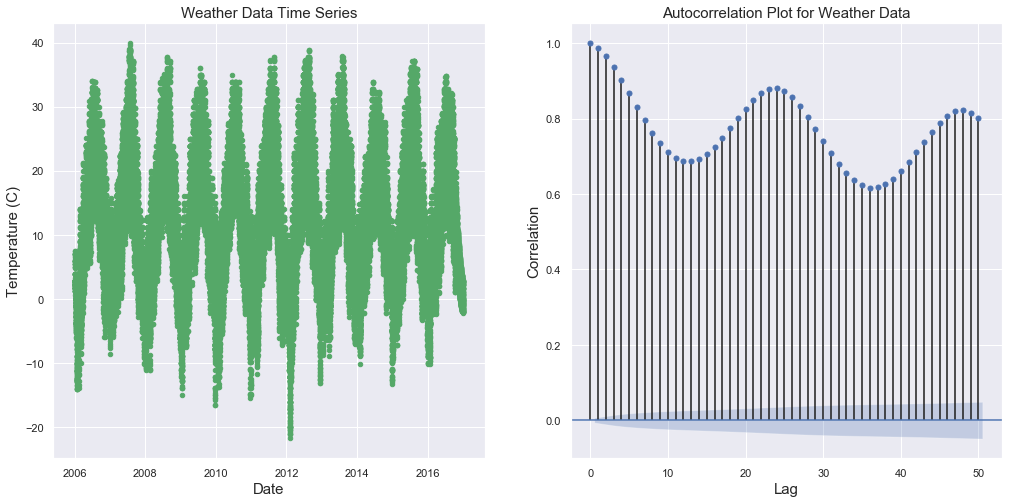

We can clearly see a repeating pattern on the left which seems to have a sinusoidal shape. On the right, we can visualize the autocorrelation plot: the size of the lines indicate the amount of correlation for that given lag value. The graph seems to indicate a cyclical pattern of correlation which makes sense when we consider the seasonal and repetitive nature of the weather.

我们可以清楚地在左侧看到一个重复的模式，看起来像是一个正弦曲线形状。 在右侧，我们可以可视化自相关图：线的大小表示该给定滞后值的相关量。 该图似乎表明相关性的周期性变化，当我们考虑天气的季节性和重复性时，这是有意义的。

However, what could we expect from an autocorrelation plot for a sales dataset? Would it present the same clear repeating pattern as this simple weather dataset?

但是，从销售数据集的自相关图可以期望什么呢？ 它会提供与这个简单的天气数据集相同的清晰重复模式吗？

Let’s plot the same information as above but with this retail sales dataset.

让我们用上述零售数据集来绘制与上述相同的信息。

The steps here will be:

这里的步骤将是：

• Load the dataset
  加载数据集
• Get the total volume of sales for 45 stores
  获取45家商店的总销售量
• Plot the total volume of sales between 2010 and 2013
  绘制2010年至2013年之间的总销量

import pandas as pd
import matplotlib.pyplot as plt
import seaborn as sns
sns.set()
from statsmodels.graphics.tsaplots import plot_acf
import matplotlib.dates as mdates
import datetimegreen = sns.color_palette("deep",8)[2]
blue = sns.color_palette("deep",8)[0]
retail_sales = "./sales_dataset.csv'
df_sales  = pd.read_csv(retail_sales)fig = plt.figure(figsize=(17,8))
ax1 = fig.add_subplot(121)
df_sales_sum = df_sales.groupby(by=['Date'], as_index=False)['Weekly_Sales'].sum()
df_sales_sum["Date"] = pd.to_datetime(df_sales_sum["Date"])
df_sales_sum.plot(x="Date",y="Weekly_Sales",color="g",ax=ax1, fontsize=15)
plt.xlabel("Date",fontsize=15)
plt.title("Total Sales Volume", fontsize=15)
plt.ylabel("Sales", fontsize=15)
date_form = mdates.DateFormatter("%Y-%m-%d")
year_locator = mdates.YearLocator()
ax1.xaxis.set_major_locator(year_locator)ax2 = fig.add_subplot(122)
plot_acf(df_sales_sum.Weekly_Sales,ax=ax2)
plt.title("Autocorrelation", fontsize=15)
plt.xlabel("Lag",fontsize=15)
plt.ylabel("Correlation", fontsize=15)
plt.show()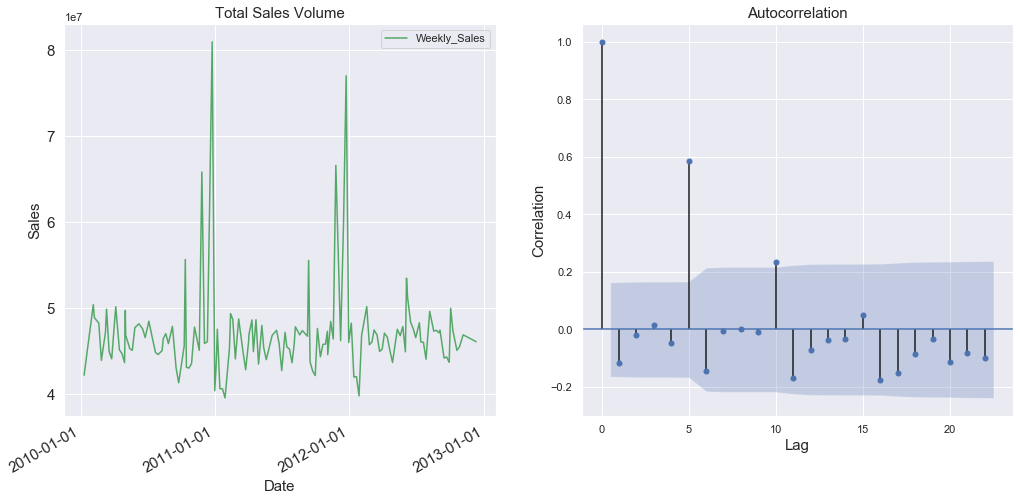

Here we see one point of relatively high correlation on an observation at lag = 5. The lack of the same structure we saw in the previous graph is a result of the contingencies of sales: given the number of factors that go into predicting sales, we should not expect the data to have perfectly clear correlations as in the weather dataset. However, it's interesting to observe spikes of correlation that could be associated with factors that relate to the type of product involved. For example, for a store that sells Christmas gifts, we should expect to see high correlation between the observations separated one year apart starting from Christmas, because people are more likely to buy more gifts during this particular period.

在这里，我们在lag = 5观察到了一个相对较高的相关点。 我们在上一张图中看到的相同结构的缺乏是由于销售的偶然性：鉴于预测销售的因素数量众多，我们不应该期望数据像天气数据集那样具有完全清晰的相关性。 然而，有趣的是观察到相关峰值可能与涉及所涉及产品类型的因素有关。 例如，对于一家销售圣诞节礼物的商店，我们应该期望看到从圣诞节开始间隔一年的观察结果之间存在高度相关性，因为在此特定时期人们更有可能购买更多礼物。

静态模式 (Static patterns)

As the expression suggests, the concept of a static pattern relates to the idea of something that does not change.

如表达式所暗示的，静态模式的概念与不变的事物的概念有关。

In time series, the most famous proxy for this concept is stationarity, which refers to the statistical properties of a time series that remain static: the observations in a stationary time series are not dependent on time.

在时间序列中，此概念最著名的代表是平稳性 ，它是指保持静态的时间序列的统计属性：固定时间序列中的观测值不依赖于时间。

The trend and seasonality will affect the value of the time series at different times. Traditionally, we would be looking for consistency over time, for example by using the mean or the variance of the observations. When a time series is stationary, it can be easier to model and statistical modeling methods usually assume or require the time series to be stationary.

趋势和季节性会影响不同时间的时间序列值。 传统上，我们会随着时间的流逝寻找一致性，例如，使用观测值的均值或方差。 当时间序列是固定的时，建模起来会更容易，而统计建模方法通常会假定或要求时间序列是固定的。

If you want to dig deeper into stationarity I recommend this piece by Shay Palachy

如果你想更深入地平稳，我建议这一块由吉文Palachy

The standard procedure to check if a dataset is stationary involves using a test called the Dickey-Fuller test, which checks for the confidence of whether or not the data has static statistical properties. To go into more detail check this article.

检查数据集是否固定的标准过程涉及使用称为Dickey-Fuller测试的测试，该测试检查数据是否具有静态统计属性的置信度。 要更详细地检查这篇文章 。

from statsmodels.tsa.stattools import adfuller
adf_test_sales = adfuller(list(df_sales_sum["Weekly_Sales"]))
adf_test_weather = adfuller(list(df_weather["Temperature (C)"]))
print("Weather Results:")
print("ADF = " + str(adf_test_weather[0]))
print("p-value = " +str(adf_test_weather[1]))
print("Retail sales results:")
print("ADF = " + str(adf_test_sales[0]))
print("p-value = " +str(adf_test_sales[1]))Weather Results:
ADF = -10.140083406906376
p-value = 8.46571984130497e-18
Retail sales results:
ADF = -2.6558148827720887
p-value = 0.08200123056783876

Here, we can see that the result of the test for the weather dataset is pointing to stationary, which is a result we should take with a grain of salt because it depends heavily on how we sample our data, usually climate data is cyclo-stationary. On our retail sales dataset, however, the p-value, indicating a non-significant confidence that the data would be stationary.

在这里，我们可以看到天气数据集的测试结果指向平稳状态，这是我们应该放一粒盐的结果，因为这很大程度上取决于我们对数据进行采样的方式，通常气候数据是循环平稳的。 但是，在我们的零售数据集上，p值表示对数据将保持不变的非显着置信度。

发展趋势 (Trends)

A trend represents a tendency identified in our data. In a stock market scenario, this could be the trend of a given stock that appears to be going up or down. For Sales Forecasting, this is key: identifying a trend allows us to know the direction that our time-series is heading, which is fundamental for predicting the future of sales.

趋势代表在我们的数据中确定的趋势。 在股票市场情况下，这可能是给定股票似乎在上涨或下跌的趋势。 对于销售预测，这是关键： 确定趋势可以使我们知道时间序列的前进方向，这是预测销售未来的基础。

We will use the fbprophet package to identify the overall trends for both our datasets. The steps will be:

我们将使用fbprophet包来识别两个数据集的总体趋势。 步骤将是：

• Select a range for the weather data (between 2007 and 2009)
  选择天气数据的范围(2007年至2009年之间)

• Feed the data to the fbprophet.Prophet object as a dataframe with two columns: "ds" (for date) and "y" (data)

  将数据作为具有两列的数据帧馈入fbprophet.Prophet对象：“ ds”(用于日期)和“ y”(数据)

• Run the model
  运行模型
• Plot the trend with an upper and lower bound
  用上下限绘制趋势图

from fbprophet import Prophet
from datetime import datetime
start_date = "2007-01-01"
end_date = "2008-12-31"
df_weather["Formatted Date"] = pd.to_datetime(df_weather["Formatted Date"], utc=True)
date_range = (df_weather["Formatted Date"] > start_date) & (df_weather["Formatted Date"] < end_date)
df_prophet = df_weather.loc[date_range]
m = Prophet()
ds = df_prophet["Formatted Date"].dt.tz_localize(None)
y = df_prophet["Temperature (C)"]
df_for_prophet = pd.DataFrame(dict(ds=ds,y=y))
m.fit(df_for_prophet)
future = m.make_future_dataframe(periods=120)
forecast = m.predict(future)
forecast = forecast[["ds","trend", "trend_lower", "trend_upper"]]
fig = m.plot_components(forecast,plot_cap=False)
trend_ax = fig.axes[0]
trend_ax.plot()
plt.title("Trend for Weather Data", fontsize=15)
plt.xlabel("Date", fontsize=15)
plt.ylabel("Weather Trend", fontsize=15)
plt.show()INFO:fbprophet:Disabling yearly seasonality. Run prophet with yearly_seasonality=True to override this.
C:\Users\lucas\.conda\envs\env_1\lib\site-packages\pystan\misc.py:399: FutureWarning:
Conversion of the second argument of issubdtype from `float` to `np.floating` is deprecated. In future, it will be treated as `np.float64 == np.dtype(float).type`.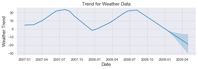

We can see that for the weather, the trend follows the regular seasons as we would expect, going up during the summer and down during the winter.

我们可以看到，对于天气，趋势遵循了我们预期的常规季节，夏季上升，冬季下降。

Now, let’s do the same for the retail dataset. The steps will be similar to the ones for the above plot, with the only difference being that here we will select one store from the retail dataset.

现在，让我们对零售数据集执行相同的操作。 步骤将与上面的图解相似，唯一的区别是在这里我们将从零售数据集中选择一家商店。

from fbprophet import Prophet
m = Prophet()
# Selecting one store
df_store_1 = df_sales[df_sales["Store"]==1]
df_store_1["Date"] = pd.to_datetime(df_store_1["Date"])
ds = df_store_1["Date"].dt.tz_localize(None)
y = df_store_1["Weekly_Sales"]
df_for_prophet = pd.DataFrame(dict(ds=ds,y=y))
m.fit(df_for_prophet)
future = m.make_future_dataframe(periods=15)
forecast = m.predict(future)
forecast = forecast[["ds","trend", "trend_lower", "trend_upper"]]
fig = m.plot_components(forecast,plot_cap=False)
trend_ax = fig.axes[0]
trend_ax.plot()
plt.title("Trend for Retail Data", fontsize=15)
plt.xlabel("Date", fontsize=15)
plt.ylabel("Sales Trend", fontsize=15)
plt.show()C:\Users\lucas\.conda\envs\env_1\lib\site-packages\ipykernel_launcher.py:8: SettingWithCopyWarning:
A value is trying to be set on a copy of a slice from a DataFrame.
Try using .loc[row_indexer,col_indexer] = value instead
See the caveats in the documentation: https://pandas.pydata.org/pandas-docs/stable/user_guide/indexing.html#returning-a-view-versus-a-copy
INFO:fbprophet:Disabling daily seasonality. Run prophet with daily_seasonality=True to override this.
C:\Users\lucas\.conda\envs\env_1\lib\site-packages\pystan\misc.py:399: FutureWarning:
Conversion of the second argument of issubdtype from `float` to `np.floating` is deprecated. In future, it will be treated as `np.float64 == np.dtype(float).type`.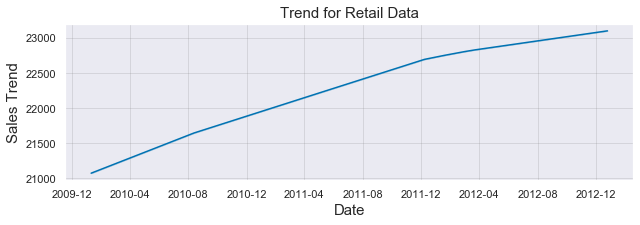

The sales performance of the selected store shows an almost perfectly linear upward trend from 2010 to 2013, showing an increase of total volume sales of over 1%. The practical interpretation of these results require other metrics like churn, and potential increase in costs, so an upward trend does not necessarily mean that the profits increased. However, the trend is a good indicator of overall performance once all the factors are considered.

从2010年到2013年，所选商店的销售业绩呈现几乎完美的线性上升趋势，显示总销量增长超过1％。 对这些结果的实际解释需要其他指标，例如客户流失和潜在的成本增加，因此上升趋势并不一定意味着利润增加。 但是，一旦考虑所有因素，趋势便是整体绩效的良好指标。

传统时间序列模型进行销售预测 (Traditional Time Series Models to Sales Forecasting)

So far, we covered the basics of the sales forecasting problem and identified the main components of it from a time series perspective: repeating patterns, static patterns and the idea of a trend. If you want to dig deeper on time series, I recommend this article by @Will Koehrsen.

到目前为止，我们介绍了销售预测问题的基础知识，并从时间序列的角度确定了该问题的主要组成部分：重复模式，静态模式和趋势概念。 如果您想更深入地了解时间序列，我建议使用@Will Koehrsen的这篇文章 。

Now we will look into the traditional time series approaches to deal with sales forecasting problems:

现在，我们将研究用于处理销售预测问题的传统时间序列方法：

• Moving Average
  移动平均线
• Exponential smoothing
  指数平滑
• ARIMA
  有马

移动平均线 (Moving Average)

This model assumes that the next observation is the mean of all past observations and it can be used to identify interesting trends in the data. We can define a window to apply the moving average model to smooth the time series, and highlight different trends.

该模型假设下一个观察值是所有过去观察值的均值，并且可以用来识别数据中有趣的趋势。 我们可以定义一个窗口来应用移动平均模型来平滑时间序列，并突出显示不同的趋势。

Let’s use the moving average model to predict the weather and sales. The steps will be:

让我们使用移动平均模型来预测天气和销售。 步骤将是：

• Select a range
  选择范围
• Define a value for our moving average window
  为我们的移动平均窗口定义一个值
• Calculate the mean absolute error
  计算平均绝对误差
• Plot an upper and lower bound for the rolling mean
  绘制滚动平均值的上限和下限
• Plot the real data
  绘制真实数据

from sklearn.metrics import mean_absolute_error
green = sns.color_palette("deep", 8)[2]
blue = sns.color_palette("deep", 8)[0]
start_date = "2007-01-01"
end_date = "2008-12-31"
df_weather["Formatted Date"] = pd.to_datetime(df_weather["Formatted Date"], utc=True)
date_range = (df_weather["Formatted Date"] > start_date) & (df_weather["Formatted Date"] < end_date)
df_weather_ma = df_weather.loc[date_range]
series = df_weather_ma["Temperature (C)"]
window=90
rolling_mean = series.rolling(window=window).mean()
fig,ax = plt.subplots(figsize=(17,8))
plt.title('Moving Average Model for Weather Dataset',fontsize=15)
plt.plot(rolling_mean, color=green, label='Rolling mean trend')
#Plot confidence intervals for smoothed values
mae = mean_absolute_error(series[window:], rolling_mean[window:])
deviation = np.std(series[window:] - rolling_mean[window:])
lower_bound = rolling_mean - (mae + 2 * deviation)
upper_bound = rolling_mean + (mae + 2 * deviation)
plt.plot(upper_bound, 'r--', label='Upper bound / Lower bound')
plt.plot(lower_bound, 'r--')
plt.plot(series[window:],color=blue, label="Actual Values")
plt.legend(loc='best')
plt.grid(True)
plt.xticks([])
plt.show()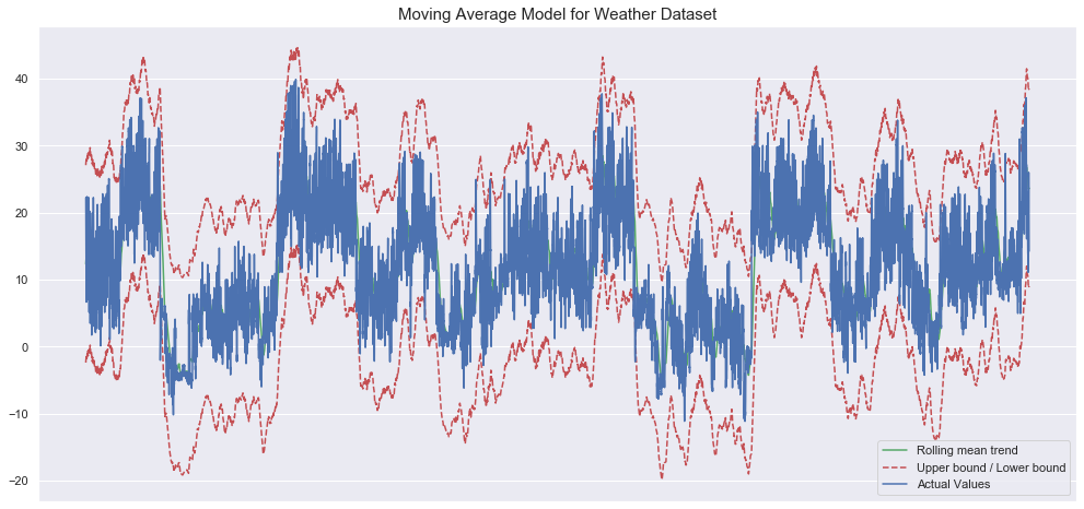

The model seems to capture some of the dynamics of the weather. Let’s see how the model does with the retail dataset.

该模型似乎捕获了一些天气动态。 让我们看看该模型如何处理零售数据集。

series = df_sales_sum.Weekly_Sales
window=15
rolling_mean = series.rolling(window=window).mean()
fig,ax = plt.subplots(figsize=(17,8))
plt.title('Moving Average Model for Retail Sales',fontsize=15)
plt.plot(rolling_mean, color=green, label='Rolling mean trend')
#Plot confidence intervals for smoothed values
mae = mean_absolute_error(series[window:], rolling_mean[window:])
deviation = np.std(series[window:] - rolling_mean[window:])
lower_bound = rolling_mean - (mae + 1.92 * deviation)
upper_bound = rolling_mean + (mae + 1.92 * deviation)
plt.plot(upper_bound, 'r--', label='Upper bound / Lower bound')
plt.plot(lower_bound, 'r--')
plt.plot(series[window:], color=blue,label='Actual values')
plt.legend(loc='best')
plt.grid(True)
plt.xticks([])
plt.show()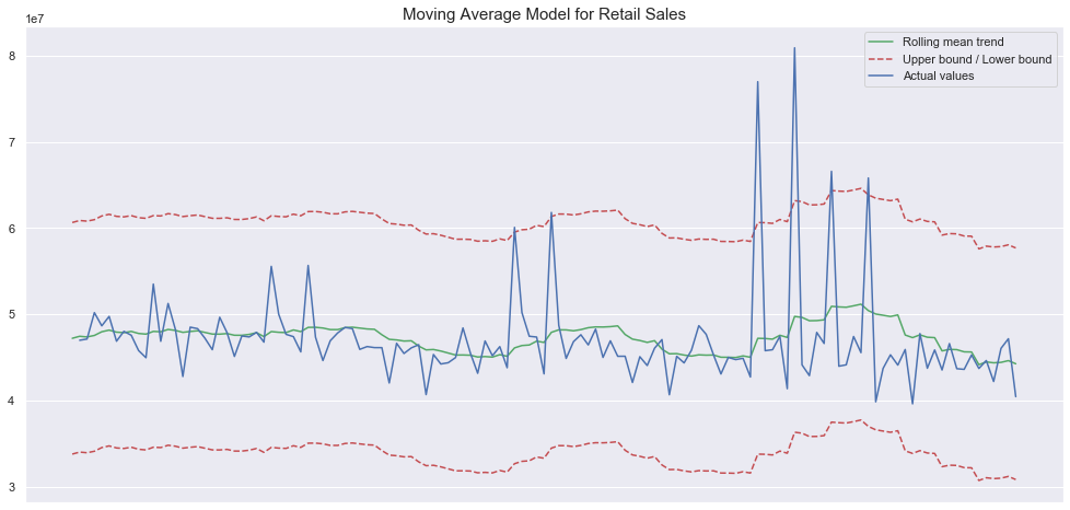

For the sales dataset, the fit does not look so promising, but the retail dataset also has much less data in comparison to the weather dataset. Additionally, the window parameter that sets the size of our averaging has a big effect on our overall performance and I did not do any additional hyper-parameter tuning. Here, what we should take away is that complex sales datasets will require more information than what a simple unidimensional time-series can provide.

对于销售数据集，拟合看起来不太理想，但与天气数据集相比，零售数据集的数据也少得多。 另外，设置平均大小的window参数对我们的整体性能有很大的影响，我没有做任何其他的超参数调整。 在这里，我们应该去除的是，复杂的销售数据集将需要比简单的一维时间序列所能提供的更多信息。

指数平滑 (Exponential Smoothing)

Exponential smoothing is similar to moving average, but in this case a decreasing weight is assigned to each observation, so less importance is given to observations as we move further from the present. Such an assumption can be good and bad: it can be beneficial to decrease the weight of outdates information within the time-series dynamics, but it can be harmful when past information has some kind of permanent causal relationship with the dynamics of the data.

指数平滑与移动平均相似，但是在这种情况下，每个观察值的权重都减小了，因此随着我们离现在越来越远，对观察值的重视程度就降低了。 这样的假设是好是坏：在时间序列动态范围内减少过时信息的权重可能是有益的，但在过去的信息与数据动态范围具有某种永久因果关系时，则可能是有害的。

Let’s use exponential smoothing in the weather dataset used above, we will:

让我们在上面使用的天气数据集中使用指数平滑，我们将：

• Fit the data
  拟合数据
• Forecast
  预测
• Plot the prediction against the real values
  根据实际值绘制预测

from statsmodels.tsa.api import ExponentialSmoothing
import matplotlib.pyplot as plt
import matplotlib.dates as mdates
import seaborn as sns
sns.set()
import pandas as pd
fit1 = ExponentialSmoothing(df_weather["Temperature (C)"][0:200]).fit(smoothing_level=0.1, optimized=False)
fit2 = ExponentialSmoothing(df_weather["Temperature (C)"][0:200]).fit(smoothing_level=0.5, optimized=False)
forecast1 = fit1.forecast(3).rename(r'$\alpha=0.1$')
forecast2 = fit2.forecast(3).rename(r'$\alpha=0.5$')
plt.figure(figsize=(17,8))
forecast1.plot(color='blue', legend=True)
forecast2.plot(color='red', legend=True)
df_weather["Temperature (ºC)"][0:200].plot(marker='',color='green', legend=True)
fit1.fittedvalues.plot(color='blue')
fit2.fittedvalues.plot(color='red')
plt.title("Exponential Smoothing for Weather Data", fontsize=15)
plt.xticks([])
plt.show()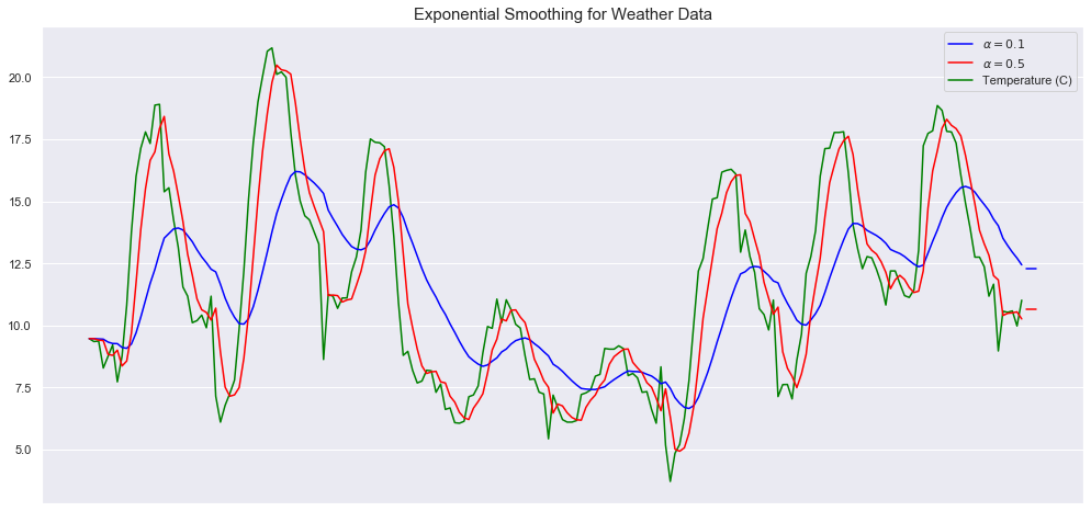

Now for the retail dataset:

现在对于零售数据集：

# Put the correct dataframe here!
fit1 = ExponentialSmoothing(df_sales_sum["Weekly_Sales"][0:200]).fit(smoothing_level=0.1, optimized=False)
fit2 = ExponentialSmoothing(df_sales_sum["Weekly_Sales"][0:200]).fit(smoothing_level=0.5, optimized=False)
forecast1 = fit1.forecast(3).rename(r'$\alpha=0.1$')
forecast2 = fit2.forecast(3).rename(r'$\alpha=0.5$')
plt.figure(figsize=(17,8))
forecast1.plot(color='blue', legend=True)
forecast2.plot(color='red', legend=True)
df_sales_sum["Weekly_Sales"][0:200].plot(marker='',color='green', legend=True)
plt.ylabel("Sales", fontsize=15)
fit1.fittedvalues.plot(color='blue')
fit2.fittedvalues.plot(color='red')
plt.title("Exponential Smoothing for Retail Data", fontsize=15)
plt.xticks([], minor=True)
plt.show()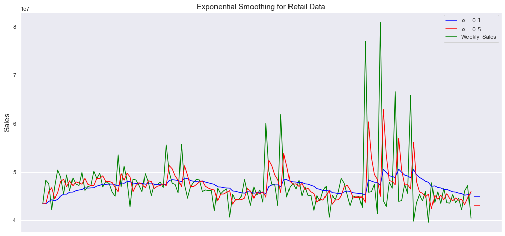

Here we are smoothing with two values for the smoothing factor (the weight of the most recent period) alpha = 0.1 and alpha = 0.5, and plotting the real temperature and retail data in green.

在这里，我们使用两个平滑值因子(最近周期的权重)α= 0.1和alpha = 0.5进行平滑，并以绿色绘制实际温度和零售数据。

As we can see here, the smaller the smoothing factor, the smoother the time series will be. This makes intuitive sense, because as the smoothing factor approaches 0, we approach the moving average model. The first one seems to capture well the dynamics on both datasets yet it seems to fail to capture the magnitude of certain peak activities.

如我们在这里看到的，平滑因子越小，时间序列将越平滑。 这很直观，因为当平滑因子接近0时，我们接近移动平均模型。 第一个似乎很好地捕捉了两个数据集的动态，但似乎未能捕捉到某些高峰活动的幅度。

Conceptually, it is interesting to reflect on how an assumption of a model can shape its performance given the nature of a dataset. I can be expected that new information is more important for sales because the factors that affect the likelihood of a store selling a product are probably changing and being updated constantly. Therefore, a model that has the capability of decreasing the importance of past information would capture this shifting dynamics more accurately when compared to one that assumes the dynamics are kept somehow constant.

从概念上讲，考虑到数据集的性质，思考模型的假设如何影响其性能是很有趣的。 可以预料，新信息对销售更重要，因为影响商店销售产品可能性的因素可能会发生变化并不断更新。 因此，与假设动态保持某种恒定程度的模型相比，具有降低过去信息重要性的能力的模型将更准确地捕获这种变化的动态。

有马 (Arima)

ARIMA or Auto-regressive Integrated Moving Average is a time series model that aims to describe the auto-correlations in the time series data. It works well for short-term predictions and it can be useful to provide forecasted values for user-specified periods showing good results for demand, sales, planning, and production.

ARIMA或自回归综合移动平均线是一个时间序列模型，旨在描述时间序列数据中的自相关。 它适用于短期预测，并且可以为用户指定的时期提供预测值，显示出对需求，销售，计划和生产的良好结果。

The parameters of the ARIMA model are defined as follows:

ARIMA模型的参数定义如下：

• p: The number of lag observations included in the model
  p：模型中包含的滞后观察次数
• d: The number of times that the raw observations are differenced
  d：原始观测值相差的次数
• q: The size of the moving average window
  q：移动平均窗口的大小

Now I am going to use ARIMA model to model the weather data and retail sales. The steps will be:

现在，我将使用ARIMA模型对天气数据和零售销售进行建模。 步骤将是：

• Split the data into training and testing
  将数据分为训练和测试
• Fit the data
  拟合数据
• Print the mean square error (our evaluation metric)
  打印均方误差(我们的评估指标)
• Plot the model fit with the real values
  用真实值绘制模型拟合

from statsmodels.tsa.arima_model import ARIMA
from sklearn.metrics import mean_squared_error
import pandas as pd
X = df_weather["Temperature (C)"].values
train_size = 600
test_size = 200
train, test = X[0:train_size], X[train_size:train_size+test_size]
history = [x for x in train]
predictions = []
for t in range(len(test)):
	model = ARIMA(history, order=(5,1,0))
	model_fit = model.fit(disp=0)
	output = model_fit.forecast()
	yhat = output[0]
	predictions.append(yhat)
	obs = test[t]
	history.append(obs)
mse = mean_squared_error(test, predictions)
print(f"MSE error: {mse}")
plt.figure(figsize=(17,8))
plt.plot(test)
plt.plot(predictions, color='red')
plt.title("ARIMA fit Weather Data")
plt.xticks([])
plt.show()MSE error: 3.105596078192541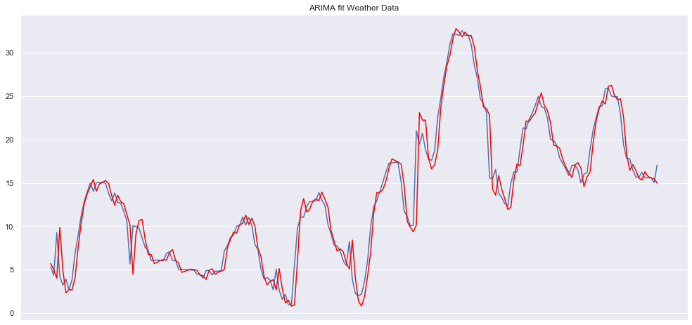

Here, we see an expected good fit of the ARIMA model to the weather dataset given that before we saw that this dataset had really high autocorrelation. Let’s compare this with how the model behaves with the sales dataset:

在这里，我们可以看到ARIMA模型与天气数据集的预期良好拟合，因为在我们看到该数据集具有很高的自相关之前。 让我们将此与模型与销售数据集的行为进行比较：

from statsmodels.tsa.arima_model import ARIMA
from sklearn.metrics import mean_squared_error
import pandas as pd
import matplotlib.pyplot as plt
import seaborn as sns
sns.set()
X = df_sales_sum["Weekly_Sales"].values
split = int(0.66*len(X))
train, test = X[0:split], X[split:]
history = [x for x in train]
predictions = []
for t in range(len(test)):
	model = ARIMA(history, order=(5,1,0))
	model_fit = model.fit(disp=0)
	output = model_fit.forecast()
	yhat = output[0]
	predictions.append(yhat)
	obs = test[t]
	history.append(obs)
mse = mean_squared_error(test, predictions)
print(f"MSE error: {mse}")
plt.figure(figsize=(17,8))
plt.plot(test)
plt.plot(predictions, color='red')
plt.title("ARIMA fit to Sales Data",fontsize=15)
plt.xticks([])
plt.show()MSE error: 47664398980324.34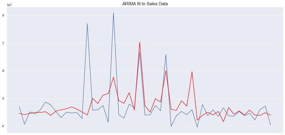

Here, the fit is not nearly as good as it was in the weather dataset which is to be expected given that the ARIMA model usually works well for datasets that are highly stationary.

在这里，拟合度不如在气象数据集中要好，这是可以预期的，因为ARIMA模型通常对于高度固定的数据集工作得很好。

Let’s just remember that the results here are merely to showcase the models and do not represent an accurate estimate. The datasets are limited (the retail sales dataset after summing is smaller than 200 data points) and I did not perform any complex hyperparameter tuning. The goal here was just to demonstrate how these models work and how they can be implemented in python. We can verify that the retail dataset seems to present challenges that the traditional models fail to overcome.

让我们记住，这里的结果只是为了展示模型，并不代表准确的估计。 数据集有限(求和后的零售数据集小于200个数据点)，我没有执行任何复杂的超参数调整。 这里的目的只是演示这些模型如何工作以及如何在python中实现它们。 我们可以验证零售数据集似乎提出了传统模型无法克服的挑战。

We can see that, for datasets that have a clear pattern, traditional models work well. However, in the absence of such a structure, these models don’t seem to present the flexibility to adapt because they rely on strong assumptions regarding the dynamics of the target time-series.

我们可以看到，对于具有清晰模式的数据集，传统模型效果很好。 但是，在没有这种结构的情况下，这些模型似乎没有提供适应的灵活性，因为它们依赖于有关目标时间序列动态的强大假设。

Now, we will discuss the current deep learning approaches to sales forecasting and try to understand what they could bring to the table that would be beneficial for forecasting accuracy in situations where traditional models are not enough.

现在，我们将讨论当前用于销售预测的深度学习方法，并尝试了解它们可以带来哪些好处，这将有助于在传统模型不足的情况下预测准确性。

现代销售预测和深度学习 (Modern Sales Forecasting and Deep Learning)

Here I want to outline the main candidates of what I believe to be the most suitable deep learning candidates for sales forecasting.

在这里，我想概述一下我认为最适合用于销售预测的深度学习候选人的主要候选人。

亚马逊的DeepAR模型 (Amazon’s DeepAR model)

The models we discussed here today fit a single model to each individual time series. However, in sales, there are often multiple time series that relate to the dynamics you are trying to model. For this reason, it is extremely beneficial to be able to jointly train a model over all the relevant time series.

我们今天在这里讨论的模型将单个模型适合每个单独的时间序列。 但是，在销售中，通常有多个时间序列与您要建模的动力学相关。 因此，能够在所有相关时间序列上共同训练模型非常有益。

Enters Amazon Forecast DeepAR+, a supervised learning algorithm that uses recurrent neural networks to forecast one-dimensional time series. It allows for training multiple time series features on one model and it outperforms the traditional models on the standard time series benchmarks.

进入Amazon Forecast DeepAR +，这是一种监督学习算法，该算法使用递归神经网络预测一维时间序列。 它允许在一个模型上训练多个时间序列特征，并且在标准时间序列基准上优于传统模型。

The main point about this model is that it overcomes one of the limitations of traditional models that can only be trained on a single time series. In addition, the model uses probabilistic forecasts, where, instead of a traditional point forecast of how much we expect to sell on a given day or period, the model predicts the distribution of the likelihoods of different future scenarios showcasing a set of prediction intervals. These prediction quantiles can be used to express the uncertainty in the forecasts and therefore give us a confidence interval for each prediction. These kinds of forecasts are specially important when it comes to downstream usage decisions where point forecasts have little use.

关于此模型的要点是，它克服了只能在单个时间序列上进行训练的传统模型的局限性之一。 此外，该模型使用概率预测 ，在该模型中，我们用传统的预测点来预测给定日期或期间的销售量，而不是预测一组集合预测间隔的不同未来方案的可能性分布。 这些预测分位数可用于表达预测中的不确定性，因此可为我们提供每个预测的置信区间。 当涉及点预测很少使用的下游使用决策时，这类预测特别重要。

NLP销售预测 (NLP for Sales Forecasting)

One approach that seems unconventional at first but holds much promise is using Natural Language Processing models to make forecasting predictions. There are two approaches that I want to mention:

乍一看似乎非常规但有很大希望的一种方法是使用自然语言处理模型进行预测。 我想提到两种方法：

• Sales Forecasting with entity embeddings

  具有实体嵌入的销售预测

• Sales Forecasting from language of product descriptions

  使用产品描述语言进行销售预测

Entity Embeddings

实体嵌入

In this article by LotusLabs they describe an idea to use categorical data (data that is unrelated to each other) and leverage an embedding representation of this data to make predictions. To build this representation conventional neural networks were used to map inputs to the embedding space.

在LotusLabs的这篇文章中，他们描述了使用分类数据(彼此不相关的数据)并利用该数据的嵌入表示来进行预测的想法。 为了建立这种表示，使用传统的神经网络将输入映射到嵌入空间。

By identifying similar inputs and mapping them to a similar location, they were able to identify patterns that would otherwise have been difficult to see. One of the advantages of using such an approach is that you don’t have to perform any feature engineering.

通过识别相似的输入并将它们映射到相似的位置，他们能够识别原本很难看到的模式。 使用这种方法的优点之一是您不必执行任何功能工程。

An interesting detail about this approach is that it overcomes issues like sparsity in simple one-hot-encoding representations.

关于此方法的一个有趣的细节是，它克服了简单的单热编码表示中的稀疏性等问题。

NLP on Product Descriptions to Forecast Sales

关于预测销售的产品描述的NLP

This paper took a different approach. They used data from more than 90,000 product descriptions on the Japanese e-commerce marketplace Rakuten and identified actionable writing styles and word usages that were highly predictive of consumer purchasing behavior.

本文采用了不同的方法。 他们使用了来自日本电子商务市场Rakuten上超过90,000种产品描述的数据，并确定了可以预测消费者购买行为的可行的写作风格和词语用法。

The model used a combination of word vectors, LSTMs and attention mechanisms to predict sales. They discovered that seasonal, polite, authoritative and informative product descriptions led to the best outcomes.

该模型结合了词向量，LSTM和注意力机制来预测销售。 他们发现季节性，礼貌，权威和信息丰富的产品描述可带来最佳效果。

Besides, they showed that words in the embedded narratives of product descriptions are very important determinants of sales even when you take into account other elements like brand loyalty and item identity. Their novel feature selection method using neural networks had good performance and the approach itself points to the heterogeneity of the dataset landscape that one must consider when using performing sales forecasting.

此外，他们还表明，即使您考虑到品牌忠诚度和商品标识等其他因素，产品说明中嵌入的文字也是决定销售的重要因素。 他们使用神经网络的新颖特征选择方法具有良好的性能，该方法本身指出了在执行销售预测时必须考虑的数据集格局的异质性。

WAVENET for Sales Forecasting

WAVENET用于销售预测

The second place at the Corporacion Favorita Grocery Sales Forecasting competition used an adapted version of the Wavenet CNN model . Wavenet is a generative model that can generate sequences of real-valued data given some conditional inputs. According to the authors, the main idea here lies in the concept of dilated causal convolutions.

Corporacion Favorita杂货销售预测竞赛的第二名使用Wavenet CNN模型的改进版本 。 Wavenet是一个生成模型，可以在某些条件输入的情况下生成实值数据序列。 这组作者认为，这里的主要思想在于膨胀因果卷积的概念。

WaveNet is structured as a fully convolutional neural network, where the convolutional layers have various dilation factors that allow its receptive field to grow exponentially and cover many time points using up sampled filters that can preserve the size of feature maps. This approach can increase the field of view of the kernel and capture the overall global view of the input. To read more about it I recommend this article by DeepMind.

WaveNet被构造为一个完全卷积的神经网络，其中的卷积层具有各种扩张因子，这些因子使它的接收场呈指数增长，并使用可以保留特征图大小的上采样滤波器覆盖许多时间点。 这种方法可以增加内核的视野，并捕获输入的整体全局视图。 要了解更多信息，我推荐DeepMind撰写的这篇文章 。

Generative models seem to be one clear trend within deep learning for sales forecasting, given their proven ability to model distributions and therefore allowing for predictions of the likelihood of different scenarios, which, in the contingent context of sales forecasting, seems to be a better approach than traditional models when one has access to enough data.

生成模型似乎是深度学习中用于销售预测的一个明显趋势，因为它们具有可靠的分布模型建模能力，因此可以预测不同情况的可能性，这在销售预测的偶然情况下似乎是一种更好的方法可以访问足够多数据的传统模型。

A Quick Note on Meta-Learning

元学习快速笔记

In this recent paper published in may of this year, a meta-learning approach to sales forecasting was developed by Shaohui Ma and Robert Fildes. The idea was to use meta-learners leveraging a pool of potential forecasting methods instead of a one model approach.

在今年5月发表的最新论文中，马少辉和罗伯特·菲尔德斯开发了一种用于销售预测的元学习方法。 这个想法是利用元学习者利用一组潜在的预测方法，而不是单一模型方法。

Their approach uses meta learners for extracting the relevant features of the data using a stacked sequence of 1-D convolutions and rectified linear units with pooling at the end. In the ensemble phase they join predictions from multiple forecasts using dense layers and softmax.

他们的方法使用元学习器，通过一维卷积和经过校正的线性单元(最后合并)的堆叠序列来提取数据的相关特征。 在集成阶段，它们使用密集层和softmax将来自多个预测的预测合并在一起。

Their approach points indicates a tendency of the field towards more hybrid self-learning approaches rather than single model solutions.

他们的方法论点表明该领域倾向于采用更多的混合自学习方法，而不是单一模型解决方案。

结论 (Conclusion)

Traditional methods can only account for the dynamics of the one-dimensional data they are trained on. However, approaches like this point to a future of hybrid models where multiple time series can be accounted for and categorical variables can be included in the forecasting pipeline.

传统方法只能考虑对其进行训练的一维数据的动态性。 但是，类似的方法指出了混合模型的未来，其中可以考虑多个时间序列，并且可以将分类变量包括在预测管道中。

Generality and flexibility seem to be the key factors that permeate successful sales forecasting models. Deep learning enables the development of sophisticated, customized forecasting models that incorporate unstructured retail data sets, therefore it can only make sense to use them when the data is complicated enough.

通用性和灵活性似乎是渗透成功的销售预测模型的关键因素。 深度学习可以开发包含非结构化零售数据集的复杂，定制的预测模型，因此只有在数据足够复杂时才使用它们。

If you want to check out the notebook for this post you can find it here.

如果您想查看这篇文章的笔记本，可以在这里找到。

If you liked this post connect with me on LinkedIn and Twitter.

如果您喜欢这篇文章，请通过LinkedIn和Twitter与我联系。

Thanks and see you next time! :)

谢谢，下次见！ :)