在科学研究中，从方法论上来讲，都应“先见森林，再见树木”。当前，人工智能学术研究方兴未艾，技术迅猛发展，可谓万木争荣，日新月异。对于AI从业者来说，在广袤的知识森林中，系统梳理脉络，才能更好地把握趋势。为此，我们精选国内外优秀的综述文章，开辟“综述专栏”，敬请关注。

作者：知乎—来咯兔子

地址：https://zhuanlan.zhihu.com/p/263053978

01

简介

贝叶斯神经网络不同于一般的神经网络，其权重参数是随机变量，而非确定的值。如下图所示：

也就是说，和传统的神经网络用交叉熵，mse等损失函数去拟合标签值相反，贝叶斯神经网络拟合后验分布。这样做的好处，就是降低过拟合。

02

BNN模型

BNN 不同于 DNN，可以对预测分布进行学习，不仅可以给出预测值，而且可以给出预测的不确定性。这对于很多问题来说非常关键，比如：机器学习中著名的 Exploration & Exploitation (EE)的问题，在强化学习问题中，agent 是需要利用现有知识来做决策还是尝试一些未知的东西；实验设计问题中，用贝叶斯优化来调超参数，选择下一个点是根据当前模型的最优值还是利用探索一些不确定性较高的空间。比如：异常样本检测，对抗样本检测等任务，由于 BNN 具有不确定性量化能力，所以具有非常强的鲁棒性。概率建模:

在这里，选择似然分布的共轭分布，这样后验可以分析计算。比如，beta分布的先验和伯努利分布的似然，会得到服从beta分布的后验。

由于共轭分布，需要对先验分布进行约束。因此，我们尝试使用采用和变分推断来近似后验分布。神经网络： 使用全连接网络来拟合数据，相当于使用多个全连接网络。但是神经网络容易过拟合，泛化性差；并且对预测的结果无法给出置信度。BNN: 把概率建模和神经网络结合起来，并能够给出预测结果的置信度。先验用来描述关键参数，并作为神经网络的输入。神经网络的输出用来描述特定的概率分布的似然。通过采样或者变分推断来计算后验分布。同时，和神经网络不同，权重 W 不再是一个确定的值，而是一个概率分布。BNN建模如下：假设 NN 的网络参数为 ， 是参数的先验分布，给定观测数据 ，这里  是输入数据， 是标签数据。BNN 希望给出以下的分布：也就是我们预测值为：由于，是随机变量，因此，我们的预测值也是个随机变量。其中：这里  是后验分布， 是似然函数， 是边缘似然。从公式(1)中可以看出，用 BNN 对数据进行概率建模并预测的核心在于做高效近似后验推断，而 变分推断 VI 或者采样是一个非常合适的方法。如果采样的话：我们通过采样后验分布 来评估  , 每个样本计算 , 其中 f 是我们的神经网络。正是我们的输出是一个分布，而不是一个值，我们可以估计我们预测的不确定度。

03

基于变分推断的BNN训练

如果直接采样后验概率  来评估 的话，存在后验分布多维的问题，而变分推断的思想是使用简单分布去近似后验分布。表示, 每个权重  从正态分布 中采样。希望  和  相近，并使用 KL 散度来度量这两个分布的距离。也就是优化：进一步推导：公式中，  表示给定正态分布的参数后，权重参数的分布；  表示给定网络参数后，观测数据的似然；  表示权重的先验，这部分可以作为模型的正则化。并且使用来表示变分下界ELBO， 也就是公式(4)等价于最大化ELBO：其中，我们需要对公式(4)中的期望进行求导，但是，这里，我们使用对权重进行重参数的技巧：其中， .于是,用 代 替  后有：也就是说，我们可以通过 多个不同的  ，求取 的平均值，来近似 KL 散度对  的求导。此外，除了对  进行重采样之外，为了保证  参数取值范围包含这个实轴，对  进行重采样，可以令，然后，,这里的  已经和原来定义的 不一样了。

04

BNN实践

算法：1、从  中采样，获得 ；2、分别计算 、 、 . 其中，计算  实际计算 , . 也就可以得到 。3、重复更新参数.

Pytorch实现：import torchimport torch.nn as nnimport torch.nn.functional as Fimport torch.optim as optimfrom torch.distributions import Normalimport numpy as npfrom scipy.stats import normimport matplotlib.pyplot as pltclass Linear_BBB(nn.Module):    """        Layer of our BNN.    """    def __init__(self, input_features, output_features, prior_var=1.):        """            Initialization of our layer : our prior is a normal distribution            centered in 0 and of variance 20.        """        # initialize layers        super().__init__()        # set input and output dimensions        self.input_features = input_features        self.output_features = output_features        # initialize mu and rho parameters for the weights of the layer        self.w_mu = nn.Parameter(torch.zeros(output_features, input_features))        self.w_rho = nn.Parameter(torch.zeros(output_features, input_features))        #initialize mu and rho parameters for the layer's bias        self.b_mu =  nn.Parameter(torch.zeros(output_features))        self.b_rho = nn.Parameter(torch.zeros(output_features))                #initialize weight samples (these will be calculated whenever the layer makes a prediction)        self.w = None        self.b = None        # initialize prior distribution for all of the weights and biases        self.prior = torch.distributions.Normal(0,prior_var)    def forward(self, input):        """          Optimization process        """        # sample weights        w_epsilon = Normal(0,1).sample(self.w_mu.shape)        self.w = self.w_mu + torch.log(1+torch.exp(self.w_rho)) * w_epsilon        # sample bias        b_epsilon = Normal(0,1).sample(self.b_mu.shape)        self.b = self.b_mu + torch.log(1+torch.exp(self.b_rho)) * b_epsilon        # record log prior by evaluating log pdf of prior at sampled weight and bias        w_log_prior = self.prior.log_prob(self.w)        b_log_prior = self.prior.log_prob(self.b)        self.log_prior = torch.sum(w_log_prior) + torch.sum(b_log_prior)        # record log variational posterior by evaluating log pdf of normal distribution defined by parameters with respect at the sampled values        self.w_post = Normal(self.w_mu.data, torch.log(1+torch.exp(self.w_rho)))        self.b_post = Normal(self.b_mu.data, torch.log(1+torch.exp(self.b_rho)))        self.log_post = self.w_post.log_prob(self.w).sum() + self.b_post.log_prob(self.b).sum()        return F.linear(input, self.w, self.b)class MLP_BBB(nn.Module):    def __init__(self, hidden_units, noise_tol=.1,  prior_var=1.):        # initialize the network like you would with a standard multilayer perceptron, but using the BBB layer        super().__init__()        self.hidden = Linear_BBB(1,hidden_units, prior_var=prior_var)        self.out = Linear_BBB(hidden_units, 1, prior_var=prior_var)        self.noise_tol = noise_tol # we will use the noise tolerance to calculate our likelihood    def forward(self, x):        # again, this is equivalent to a standard multilayer perceptron        x = torch.sigmoid(self.hidden(x))        x = self.out(x)        return x    def log_prior(self):        # calculate the log prior over all the layers        return self.hidden.log_prior + self.out.log_prior    def log_post(self):        # calculate the log posterior over all the layers        return self.hidden.log_post + self.out.log_post    def sample_elbo(self, input, target, samples):        # we calculate the negative elbo, which will be our loss function        #initialize tensors        outputs = torch.zeros(samples, target.shape[0])        log_priors = torch.zeros(samples)        log_posts = torch.zeros(samples)        log_likes = torch.zeros(samples)        # make predictions and calculate prior, posterior, and likelihood for a given number of samples        for i in range(samples):            outputs[i] = self(input).reshape(-1) # make predictions            log_priors[i] = self.log_prior() # get log prior            log_posts[i] = self.log_post() # get log variational posterior            log_likes[i] = Normal(outputs[i], self.noise_tol).log_prob(target.reshape(-1)).sum() # calculate the log likelihood        # calculate monte carlo estimate of prior posterior and likelihood        log_prior = log_priors.mean()        log_post = log_posts.mean()        log_like = log_likes.mean()        # calculate the negative elbo (which is our loss function)        loss = log_post - log_prior - log_like        return lossdef toy_function(x):    return -x**4 + 3*x**2 + 1# toy dataset we can start withx = torch.tensor([-2, -1.8, -1, 1, 1.8, 2]).reshape(-1,1)y = toy_function(x)net = MLP_BBB(32, prior_var=10)optimizer = optim.Adam(net.parameters(), lr=.1)epochs = 2000for epoch in range(epochs):  # loop over the dataset multiple times    optimizer.zero_grad()    # forward + backward + optimize    loss = net.sample_elbo(x, y, 1)    loss.backward()    optimizer.step()    if epoch % 10 == 0:        print('epoch: {}/{}'.format(epoch+1,epochs))        print('Loss:', loss.item())print('Finished Training')# samples is the number of "predictions" we make for 1 x-value.samples = 100x_tmp = torch.linspace(-5,5,100).reshape(-1,1)y_samp = np.zeros((samples,100))for s in range(samples):    y_tmp = net(x_tmp).detach().numpy()    y_samp[s] = y_tmp.reshape(-1)plt.plot(x_tmp.numpy(), np.mean(y_samp, axis = 0), label='Mean Posterior Predictive')plt.fill_between(x_tmp.numpy().reshape(-1), np.percentile(y_samp, 2.5, axis = 0), np.percentile(y_samp, 97.5, axis = 0), alpha = 0.25, label='95% Confidence')plt.legend()plt.scatter(x, toy_function(x))plt.title('Posterior Predictive')plt.show()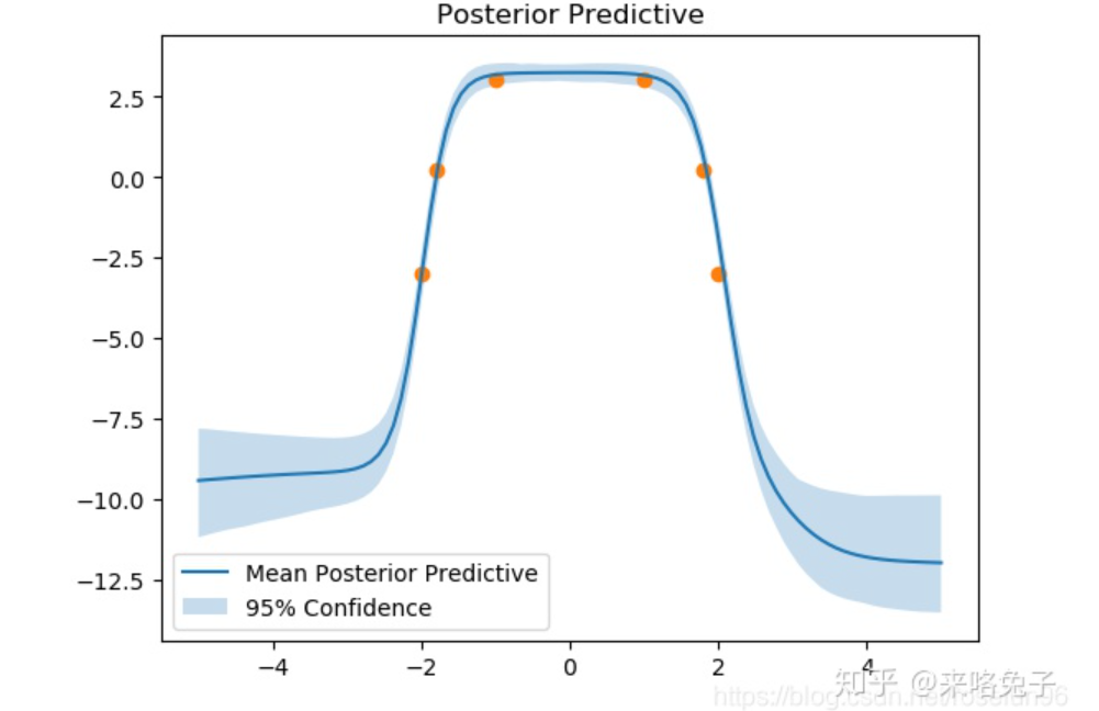

这里是重复计算100次的平均值和100次平均值的97.5%大和2.5%小的区域线图(即置信度95%)。

参考：https://mp.weixin.qq.com/s/olwyTaOGCugt-thgZm_3Mghttps://arxiv.org/ftp/arxiv/papers/1801/1801.07710.pdf

本文目的在于学术交流，并不代表本公众号赞同其观点或对其内容真实性负责，版权归原作者所有，如有侵权请告知删除。

直播预告

“综述专栏”历史文章

• 2020 Pose Estimation人体骨骼关键点检测综述笔记

• 多目标跟踪(MOT)入门

• Anchor-free应用一览：目标检测、实例分割、多目标跟踪

• 语音转换Voice Conversion：特征分离技术

• Domain Adaptation基础概念与相关文章解读

• 一日看尽长安花——NLP可解释研究梳理

• 损失函数理解汇总，结合PyTorch和TensorFlow2

• 点云距离度量：完全解析EMD距离(Earth Mover's Distance)

• One Shot NAS总结

• 图神经网络与深度学习在智能交通中的应用：综述Survey

• 异质图神经网络学习笔记

• Self-supervised Learning

• 元学习综述

• 异常检测：Anomaly Detection综述

• 计算机视觉基本任务综述

更多综述专栏文章，

请点击文章底部“阅读原文”查看

分享、点赞、在看，给个三连击呗！