赛题背景

赛题以网络舆情分析为背景，要求选手根据用户的评论来对品牌的议题进行数据分析与可视化。通过这道赛题来引导常用的数据可视化图表，以及数据分析方法，对感兴趣的内容进行探索性数据分析。

赛题数据

数据源： earphone_sentiment.csv，为10000+条行业用户关于耳机的评论
使用天池实验室打比赛即可直接在notebook中挂载数据源
https://tianchi.aliyun.com/competition/entrance/531890/information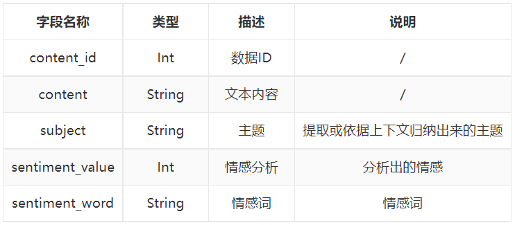

赛题任务

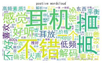
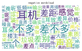
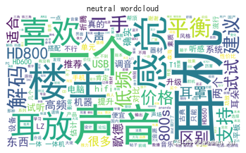
1）词云可视化（评论中的关键词，不同情感的词云）
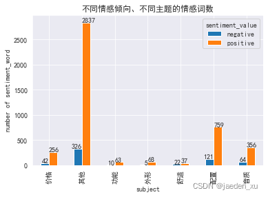
2）柱状图（不同主题，不同情感，不同情感词）
3）相关性系数热力图（不同主题，不同情感，不同情感词）
用python 做词云，需要安装两个文件包：中文分词jieba和wordcloud

1 数据探索

#导入包
import pandas as pd
import numpy as np
import jieba
import sys
from wordcloud import WordCloud,STOPWORDS
from imageio import imread
import matplotlib.pyplot as plt
import seaborn as sns
from collections import Counter

from pylab import *
plt.rcParams['font.sans-serif']=['SimHei'] 
plt.rcParams['axes.unicode_minus']=False

sns.set_style('darkgrid',{'font.sans-serif':['SimHei','DejaVa Sans']})

#导入数据
earphone_sentiment=pd.read_csv('./earphone_sentiment.csv')
earphone_sentiment

1.1 检查数据类型，并侦查重复值、缺失值

#查看重复值
print(earphone_sentiment.duplicated().sum())
#查看个字段缺失值
print(earphone_sentiment.isnull().sum())
# 查看数据字段、非空值、数据类型等
earphone_sentiment.info()

发现数据集中没有重复行，其中sentiment_word列只有4966行为非空，具有12210的大量空值，需侦查空值情况是否需处理。

数据集共17176行记录，共5个字段。

0 content_id （int64）： 数据id

1 content （object） ：文本内容

2 subject （object）：主题

3 sentiment_word （object）：情感词

4 sentiment_value （int64）：情感倾向分析

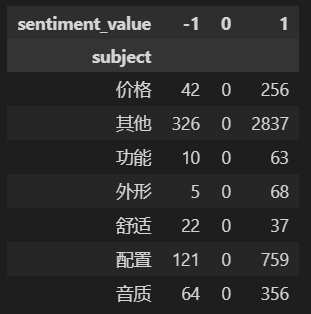
#对不同情感倾向的不同主题的情感词进行透视，查看数据
earphone_sentiment.pivot_table(columns='sentiment_value',index='subject',values='sentiment_word',aggfunc="count")

查看透视的数据可知：

1、情感倾向取值有：-1（消极情绪）,0（中性情绪）,1（积极情绪）

2、主题共有7个主题：价格、功能、外形、舒适、配置、音质、其他

3、‘sentiment_word’列所有空值属于中性情绪倾向（0）的，没有情感词，所以不做处理。

1.2 数据预处理

调取停用字典（需要剔除一些无意义的词，如：的、地、得、吗、呢、感觉、耳机、哈哈、嘻嘻、在，还有一些标点符号等等；词典可以在网上查找，也可自己建立

#读取停用词典
stop_words=[]
with open(r'./chineseStopWords.txt','r') as f:
    for line in f:
        stop_words.append(line.strip('\n').split(',')[0])

#分词
df=earphone_sentiment.copy()

row,col=df.shape  #数据表的行数
df['cutwords'] = 'cutwords'  #预定义列表

for i in np.arange(row):
    cutword = [x for x in jieba.cut_for_search(df.content[i]) if len(x) > 1]  #分词并去除长度为1的词
    cutword = [k for k in cutword if k not in stop_words]  #去除停用词
    df.cutwords[i]=cutword
    
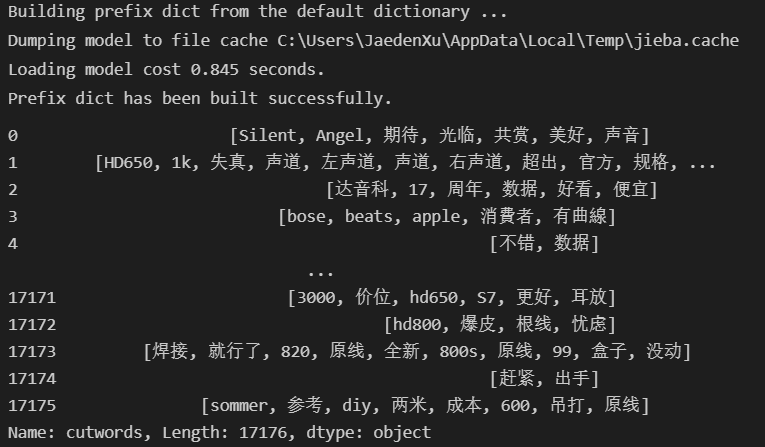
#查看全部分词结果
df.cutwords

#将情感分析分数赋值中文
new_value={-1:"negative",0:"neutral",1:"positive"}
df['sentiment_value']=df['sentiment_value'].map(new_value)

#筛选积极情绪倾向的数据
pos_df=df.loc[df['sentiment_value']=='positive']
#筛选积极情绪倾向的数据
neg_df=df.loc[df['sentiment_value']=='negative']
#筛选中性情绪倾向的数据
neu_df=df.loc[df['sentiment_value']=='neutral']

2、用户情感可视化

2.1 任务1 ：词云图可视化

（评论中的关键词、不同情感的词云）

#连接全部分词
all_text='/'.join(np.concatenate(df.cutwords))

#连接积极情绪的分词
positive_text='/'.join(np.concatenate(pos_df.cutwords.reset_index(drop=True)))

#连接消极情绪的分词
negative_text='/'.join(np.concatenate(neg_df.cutwords.reset_index(drop=True)))

#连接中性情绪的分词
neutral_text='/'.join(np.concatenate(neu_df.cutwords.reset_index(drop=True)))

#导入词云底图
earphone_mark=imread(r'./cloud.png')
pos_mark=imread(r'./cloud.png')
neu_mark=imread(r'./cloud.png')
neg_mark=imread(r'./cloud.png')

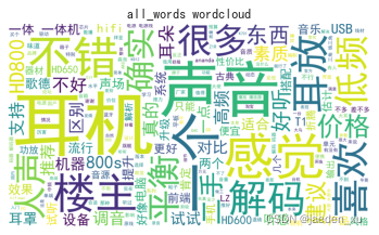
#利用文本绘制词云

#绘制总词云
wc1=WordCloud(font_path='simhei.ttf',background_color='white',margin=5,width=1800,height=800,mask=earphone_mark).generate(all_text)
plt.imshow(wc1)
plt.axis("off")
plt.title('all_words wordcloud')
plt.show()

#绘制积极情绪的词语
wc2=WordCloud(font_path='simhei.ttf',background_color='white',margin=5,width=1800,height=800,mask=pos_mark).generate(positive_text)
plt.imshow(wc2)
plt.axis("off")
plt.title('postive wordcloud')
plt.show()

#绘制消极情绪的词语
wc3=WordCloud(font_path='simhei.ttf',background_color='white',margin=5,width=1800,height=800,mask=neg_mark).generate(negative_text)
plt.imshow(wc3)
plt.axis("off")
plt.title('negative wordcloud')
plt.show()

#绘制中性情绪的词语
wc3=WordCloud(font_path='simhei.ttf',background_color='white',margin=5,width=1800,height=800,mask=neu_mark).generate(neutral_text)
plt.imshow(wc3)
plt.axis("off")
plt.title('neutral wordcloud')
plt.show()

2.2 任务2 ：柱状图

（不同主题、不同情感、不同的情感词）

2.2.1 不同情感倾向、不同主题的情感词数柱状图

#中性情绪倾向的没有情感词，剔除出来
df_vsw=df.loc[df['sentiment_value']!='neutral'].pivot_table(columns='sentiment_value',index='subject',values='sentiment_word',aggfunc="count")
print(df_vsw)

#绘制柱状图
plt.figure(figsize=(20,15))
df_vsw.plot.bar()

#标记标签（ha为位置）

for x,y in enumerate(df_vsw['negative'].values):
    plt.text(x,y,"%s" %y,ha='right') 
for x,y in enumerate(df_vsw['positive'].values):
    plt.text(x,y,"%s" %y,ha='left')
   
plt.ylabel('number of sentiment_word')
plt.title('不同情感倾向、不同主题的情感词数')
plt.show()

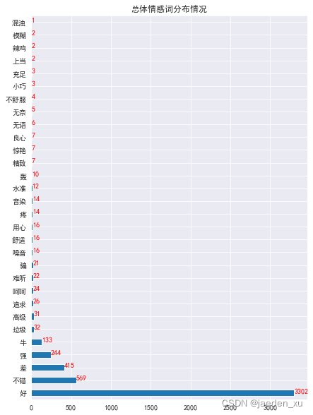
2.2.2 不同情感倾向的情感词评论数–横向柱状图

#不同情感倾向的不同情感词评论数
df2=df['sentiment_word'].value_counts()

#积极情绪的情感词评论数
df2_pos=pos_df.sentiment_word.value_counts()

#消极情绪的情感词评论数
df2_neg=neg_df.sentiment_word.value_counts()

#情感词总体分布情况
plt.figure(figsize=(7,10))
df2.plot.barh()
for y,x in enumerate(df2.values):
    plt.text(x,y,"%s" %x,color='red')
plt.title('总体情感词分布情况')
plt.show()


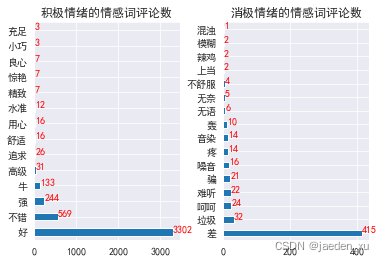
#不同情感倾向的情感词分布情况
plt.subplot(1,2,1)
df2_pos.plot.barh()
for y,x in enumerate(df2_pos.values):
    plt.text(x,y,"%s" %x,color='red')
plt.title('积极情绪的情感词评论数')

plt.subplot(1,2,2)
df2_neg.plot.barh()
for y,x in enumerate(df2_neg.values):
    plt.text(x,y,"%s" %x,color='red')
plt.title('消极情绪的情感词评论数')
plt.subplots_adjust(wspace=0.3) #调整两图水平之间距离
plt.show()

2.3 任务3：相关性系数热力图

（不同主题、不同情感、不同的情感词）

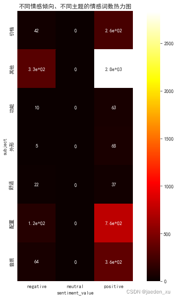
2.3.1 不同情感倾向、不同主题的情感词数–相关性热力图

df_vsw=df.pivot_table(columns='sentiment_value',index='subject',values='sentiment_word',aggfunc="count")

plt.figure(figsize=(10,10))
with sns.axes_style("white"):
    ax=sns.heatmap(df_vsw,square=True,annot=True,cmap='hot')
ax.set_title("不同情感倾向、不同主题的情感词数热力图")
plt.show()

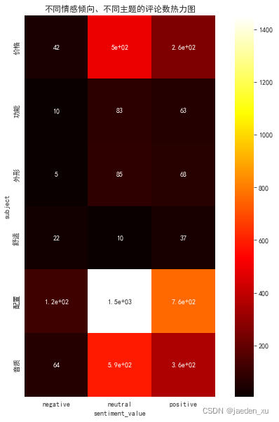
2.3.2 不同情感倾向、不同主题的评论数–相关性热力图

df_vsc=df.pivot_table(columns='sentiment_value',index='subject',values='content',aggfunc="count")
print(df_vsc)
#因“其他”主题相对来说分析意义较小，且数目过大影响热力图效果，故剔除分析
df_vsc1=df_vsc.drop("其他")

plt.figure(figsize=(10,10))
with sns.axes_style("white"):
    ax=sns.heatmap(df_vsc1,square=True,annot=True,cmap='hot')
ax.set_title("不同情感倾向、不同主题的评论数热力图")
plt.show()