Python之数据可视化
matplotlib系统介绍
https://blog.csdn.net/m0_57385293/article/details/123229485
https://www.jianshu.com/p/63ba161f0102
高等数学基于Python的实现

pyqtgraph

PyQtGraph被大量应用于Qt GUI平台（通过PyQt或PySide），因为它的高性能图形以及NumPy可用于大量数据处理。特别需要注意的是，PyQtGraph使用了Qt的GraphicsView框架，它本身是一个功能强大的图形系统，我们将优化和简化的语句应用到这个框架中，以最小的工作量实现数据可视化。

对于绘图而言，PyQtGraph几乎不像Matplotlib那么完整或者成熟，但是运行速度更快。Matplotlib的目标更多是制作出版质量的图形，而PyQtGraph则用于数据采集和分析应用。Matplotlib对于Matlab程序员来说更直观

tkinter gui绘制matplotlib图像
https://developer.aliyun.com/article/1119575
https://blog.csdn.net/football_game/article/details/103350259

matplotlib与tkinter的一些总结
https://blog.csdn.net/charie411/article/details/107365526/

Python可视化：Matplotlib基础教程
https://blog.csdn.net/u010349629/article/details/130663630

import matplotlib.pyplot as plt
import matplotlib.ticker as ticker
 
x = [1,3,5,7]
y = [4,9,6,8]
 
# 创建figure，axes，并用axes画图
figure = plt.figure()
axes = figure.add_subplot(1,1,1)
axes.plot(x,y,'o-r')
 
# x轴主刻度的位置
axes.xaxis.set_major_locator(ticker.FixedLocator([1,4,7]))
# x轴小刻度的位置
axes.xaxis.set_minor_locator(ticker.FixedLocator([2,3,5]))
 
# x轴网格（这里只设置x轴的，y轴的同理）
# 扩展参数：Line2D属性参数
axes.xaxis.grid(visible=True,
                which='major', #主刻度网格
                #扩展参数：Line2D属性参数
                color='r' #主刻度网格设置成红色以便区分
                )
axes.xaxis.grid(visible=True,
                which='minor' #小刻度网格
                #扩展参数：Line2D属性参数
                )
 
plt.show()

matplotlib.axes.Axes官方文档
https://matplotlib.org/stable/api/_as_gen/matplotlib.axes.Axes.legend.html
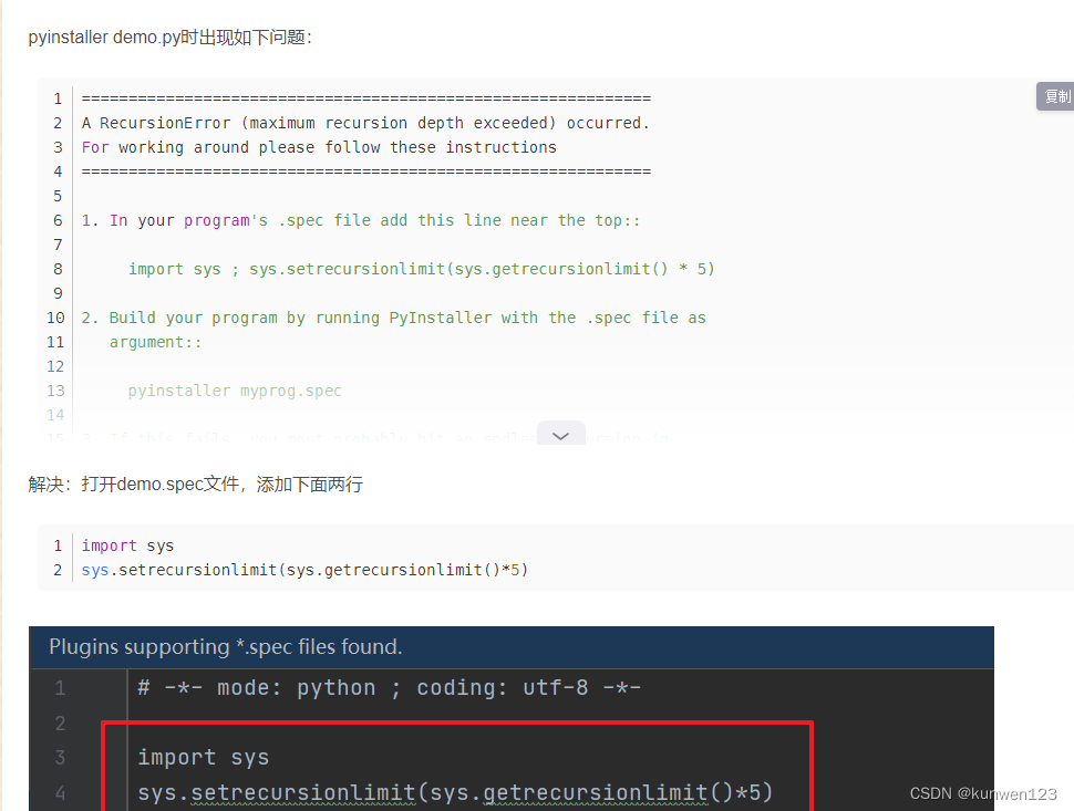
tkinter - 使用Pyinstall进行打包封装

pip install pyinstaller

Pyinstaller -F setup.py 打包exe

Pyinstaller -F -w setup.py 不带控制台的打包

Pyinstaller -F -i xx.ico setup.py 指定exe图标打包

Pyinstaller -F -w -i xx.ico setup.py 指定exe图标并且不带控制台的打包

python中plot实现即时数据动态显示
https://blog.csdn.net/u013468614/article/details/58689735
https://www.shouxicto.com/article/2540.html
https://blog.csdn.net/u013468614/article/details/104817578
https://blog.csdn.net/qq_36694133/article/details/127058949
https://blog.csdn.net/miracleoa/article/details/115407901
https://blog.csdn.net/river_star1/article/details/128959025
https://blog.csdn.net/u013180339/article/details/77002254
https://imagemagick.org/archive/binaries/ImageMagick-7.1.1-11-Q16-x64-dll.exe

python读写修改Excel之xlrd&xlwt&xlutils

import xlrd
from xlutils.copy import copy


# 打开 excel 文件, 带格式复制
read_book = xlrd.open_workbook("example-2021-03-09.xls", formatting_info=True)

# 复制一份
wb = copy(read_book)

# 选取第一个表单
sh1 = wb.get_sheet(0)

# 在第五行新增写入数据
sh1.write(4, 0, '2020-12-16')
sh1.write(4, 1, '高三三班')
sh1.write(4, 2, '小鱼仙倌儿')
sh1.write(4, 3, 150)
sh1.write(4, 4, 150)
sh1.write(4, 5, 150)
sh1.write(4, 6, 300)

# 选取第二个表单
sh2 = wb.get_sheet(1)

# 替换总成绩数据
sh2.write(1, 2, 100)

# 保存
wb.save('example-2021-03-09.xls')

问题出现在pycharm环境上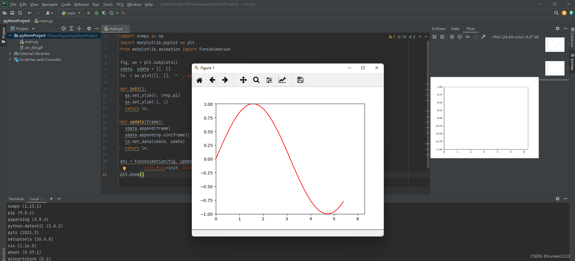

matplotlib嵌入tkinter界面并动态更新

import tkinter
import random
import tkinter as tk
import tkinter.font as tkFont
import matplotlib.pyplot as plt
from matplotlib.backends.backend_tkagg import FigureCanvasTkAgg
 
 
def generate_data():
    global vacuum, efficiency, vacuumHisList, effiHisList
    vacuum = random.uniform(-1, 0)
    efficiency = random.uniform(30, 100)
    vacuumHisList.append(vacuum)
    effiHisList.append(efficiency)
    if len(vacuumHisList) > 15:
        vacuumHisList.pop(0)
        effiHisList.pop(0)
 
    root.after(1000, generate_data)
 
def plot_efffi_vacuum():
    global vacuum, efficiency, vacuumHisList, effiHisList, fig1
 
    fig1.clf()  # 清除上一帧内容
 
    g11 = fig1.add_subplot(2, 1, 1)
    g11.plot(vacuumHisList, effiHisList, c='lawngreen')
    g11.scatter(vacuum, efficiency, c="yellow", s=30)
    g11.set_xlim([-1, 1])
    g11.set_ylim([20, 100])
    g11.set_xlabel("vacuum bar")
    g11.set_ylabel("effi %")
    g11.patch.set_facecolor('whitesmoke')
 
    g12 = fig1.add_subplot(2, 1, 2)
    g12.set_xlim([0, 120])
    g12.set_ylim([-20, 20])
    g12.set_xlabel('time s')
    g12.set_ylabel('angle deg')
    g12.patch.set_facecolor('whitesmoke')
 
    canvas.draw()
 
    root.after(1000, plot_efffi_vacuum)
 
 
def plot_fpcurve():
    pass
 
 
def plot_vacuum():
    pass
 
 
def plot_visor_angle():
    pass
 
 
def write_spc_set(x, y):
    print(x, y)
 
 
def spc_set_window():
    spc_window = tk.Toplevel()
    spc_window.title("spc set")
    spc_window.geometry("250x200")
 
    label = tk.Label(spc_window, text="Kd: ", anchor='e')
    label.place(x=0, y=0, width=80, height=30)
    text = tk.Text(spc_window, font=tkFont.Font(size=16))
    text.tag_configure("tag_name", justify='center')
    text.place(x=80, y=0, width=100, height=30)
 
    label1 = tk.Label(spc_window, text="折算系数: ", anchor='e')
    label1.place(x=0, y=50, width=80, height=30)
    text1 = tk.Text(spc_window, font=tkFont.Font(size=16))
    text1.tag_configure("tag_name", justify='center')
    text1.place(x=80, y=50, width=100, height=30)
 
    spc_confirm_btn = tk.Button(spc_window, text="Confirm", font=tkFont.Font(size=16),
                                command=lambda: write_spc_set(text.get('0.0', 'end')[:-1],
                                                              text1.get('0.0', 'end')[:-1])) #用lambda函数获取传入的参数，get 方法获取text中内容，-1去掉换行符
    spc_confirm_btn.place(x=80, y=100, width=100, height=30)
 
 
def avc_set_window():
    avc_window = tk.Toplevel()
    avc_window.title("avc set")
    avc_window.geometry("250x200")
 
    label = tk.Label(avc_window, text="真空高值: ", anchor='e')
    label.place(x=0, y=0, width=80, height=30)
    text = tk.Text(avc_window, font=tkFont.Font(size=16))
    text.tag_configure("tag_name", justify='center')
    text.place(x=80, y=0, width=100, height=30)
 
    label1 = tk.Label(avc_window, text="真空低值: ", anchor='e')
    label1.place(x=0, y=50, width=80, height=30)
    text1 = tk.Text(avc_window, font=tkFont.Font(size=16))
    text1.tag_configure("tag_name", justify='center')
    text1.place(x=80, y=50, width=100, height=30)
 
    spc_confirm_btn = tk.Button(avc_window, text="Confirm", font=tkFont.Font(size=16),
                                command=lambda: write_spc_set(text.get('0.0', 'end')[:-1],
                                                              text1.get('0.0', 'end')[:-1])) #用lambda函数获取传入的参数，get 方法获取text中内容，-1去掉换行符
    spc_confirm_btn.place(x=80, y=100, width=100, height=30)
 
 
# 定义全局变量
vacuum = 0
efficiency = 0
vacuumHisList = []
effiHisList = []
 
# 创建tkinter主界面
root = tk.Tk()
root.title("smart controller")
root.geometry("800x450+0+0")
root.configure(bg="gainsboro")
# 创建button
button_spc = tk.Button(root, text="spc设置", command=spc_set_window)
button_spc.place(x=0, y=0, width=100, height=30)
button_avc = tk.Button(root, text="avc设置", command=avc_set_window)
button_avc.place(x=100, y=0, width=100, height=30)
 
# 创建一个容器用于显示matplotlib的fig
frame1 = tk.Frame(root, bg="gainsboro")
frame1.place(x=0, y=30, width=800, height=600)
# 解决matplot中文显示乱码
plt.rcParams['font.sans-serif'] = ['SimHei']  # 防止中文标签乱码，还有通过导入字体文件的方法
plt.rcParams['axes.unicode_minus'] = False
plt.rcParams['lines.linewidth'] = 1  # 设置曲线线条宽度
# 创建画图figure
fig1 = plt.figure(figsize=(4, 4))
fig1.subplots_adjust(left=0.15, right=0.9, top=0.95, bottom=0.15, wspace=0.5, hspace=0.5)
fig1.patch.set_facecolor('gainsboro')
g11 = fig1.add_subplot(2, 1, 1)
g11.set_xlim([-1, 1])
g11.set_ylim([20, 100])
g11.set_xlabel("vacuum bar")
g11.set_ylabel("effi %")
g11.patch.set_facecolor('whitesmoke')
g12 = fig1.add_subplot(2, 1, 2)
g12.set_xlim([0, 6])
g12.set_ylim([0, 4])
g12.set_xlabel('流量 m$^3$/s')
g12.set_ylabel('产量 m$^3$/s')
g12.patch.set_facecolor('whitesmoke')
# 将fig放入画布
canvas = FigureCanvasTkAgg(fig1, master=frame1)
canvas.draw()
# 将画布放进窗口
canvas.get_tk_widget().place(x=0, y=0)
# 创建第二个图
fig2 = plt.figure(figsize=(4, 4))
fig2.subplots_adjust(left=0.2, right=0.9, top=0.95, bottom=0.15, wspace=0.5, hspace=0.5)
fig2.patch.set_facecolor('gainsboro')
g21 = fig2.add_subplot(2, 1, 1)
g21.set_xlim([0, 120])
g21.set_ylim([-1, 0])
g21.set_xlabel("time s")
g21.set_ylabel("vacuum bar")
g21.patch.set_facecolor('whitesmoke')
g22 = fig2.add_subplot(2, 1, 2)
g22.set_xlim([0, 120])
g22.set_ylim([-20, 20])
g22.set_xlabel('time s')
g22.set_ylabel('angle deg')
g22.patch.set_facecolor('whitesmoke')
# 打开matplot交互模式
plt.ion()
# fig2 放入画布
canvas2 = FigureCanvasTkAgg(fig2, master=frame1)
canvas2.draw()
canvas2.get_tk_widget().place(x=420, y=0)
# 使用一个定时器计算后台数据
generate_data()
# fig更新
plot_efffi_vacuum()
plot_fpcurve()
plot_vacuum()
plot_visor_angle()
 
root.mainloop()

Python–matplotlib（持续更新）

Python 5种经典的求积分方法

from math import *
 
 
def sgn(x):
    if x > 0:
        return 1
    elif x == 0:
        return 0
    else:
        return -1
 
 
def func(x):
    # return sgn(sin(pi / sin(x)))
    return x ** 2 + 2
 
 
def simpson(begin, between, i):
    a = begin + (i - 1) * between
    b = begin + i * between
    return between * (func(a) + func(b) + 4 * func((a + b) / 2)) / 6
 
 
def rightRectangle(begin, between, i):
    return between * func(begin + between * i)
 
 
def leftRectangle(begin, between, i):
    return between * func(begin + between * (i - 1))
 
 
def midRectangle(begin, between, i):
    return between * func(begin + between / 2 * (2 * i - 1))
 
 
def trapezoidRectangle(begin, between, i):
    return between / 2 * (func(begin + between * (i - 1)) + func(begin + between * i))
 
 
def cal_IntegralByEpsilon(begin, end, epsilon, method):
    n = 1
    result = 0
    preResult = float("inf")
    while abs(preResult - result) >= epsilon:
        preResult = result
        result = 0
        n *= 2
        between = (end - begin) / n
        for i in range(n):
            try:
                result += method(begin, between, i + 1)
            except:
                return "Integrated function has discontinuity or does not defined in current interval"
    return result
 
 
def cal_IntegralByN(begin, end, n, method):
    result = 0
    between = (end - begin) / n
    for i in range(n):
        try:
            result += method(begin, between, i + 1)
        except:
            return "Integrated function has discontinuity or does not defined in current interval"
 
 
if __name__ == "__main__":
    begin = 0.2
    end = 0.5
    epsilon = 0.0001
    print(cal_IntegralByEpsilon(begin, end, epsilon, simpson))
    print(cal_IntegralByEpsilon(begin, end, epsilon, rightRectangle))
    print(cal_IntegralByEpsilon(begin, end, epsilon, leftRectangle))
    print(cal_IntegralByEpsilon(begin, end, epsilon, midRectangle))
    print(cal_IntegralByEpsilon(begin, end, epsilon, trapezoidRectangle))
 
    begin = 0.2
    end = 0.5
    n = 10
    print(cal_IntegralByN(begin, end, n, simpson))
    print(cal_IntegralByN(begin, end, n, rightRectangle))
    print(cal_IntegralByN(begin, end, n, leftRectangle))
    print(cal_IntegralByN(begin, end, n, midRectangle))
    print(cal_IntegralByN(begin, end, n, trapezoidRectangle))

python 如何用 Python 求定积分？

import matplotlib.pyplot as plt
import numpy as np
import sympy as sy

def f(x):
    return x**2

x = sy.Symbol("x")
print(sy.integrate(f(x), (x, 0, 2)))

import matplotlib.pyplot as plt
import numpy as np

def f(x):
    return x**2

x = np.linspace(0, 2, 1000)
plt.plot(x, f(x))
plt.axhline(color="black")
plt.fill_between(x, f(x), where=[(x > 0) and (x < 2) for x in x])
plt.show()

利用Python实现数值积分的方法（有矩形方法）

import numpy as np
x = np.linspace(0, 3, 1001)
f = lambda x: x**3 - 4*x**2 + 4*x + 2
a = 0.5
b = 2.5
Ax = np.linspace(a, b, 101)
Ay = f(Ax)
def defInt_left(f, a, b, N):
    # left-hand point
    result = 0; FX = []; Xn = []
    dx = abs(b - a)/N
    while a < b:
        result += f(a)*dx
        FX += [f(a)]
        Xn += [a]
        a += dx
    return result, FX, Xn, dx
N = 4
I_left, FX, Xn, dx = defInt_left(f, a, b, N)
print(I_left)

python matplotlib.pyplot画矩形图 以及plt.gca()

import matplotlib.pyplot as plt

fig = plt.figure()
ax = fig.add_subplot(111)

rect = plt.Rectangle((0.1,0.1),0.5,0.3)
ax.add_patch(rect)

plt.show()

import matplotlib.pyplot as plt

fig = plt.figure()　　#创建图
ax = fig.add_subplot(111)  #创建子图

plt.gca().add_patch(plt.Rectangle((0.1,0.1),0.5,0.3))
plt.show()

sympy官网 中文
sympy官网 英文

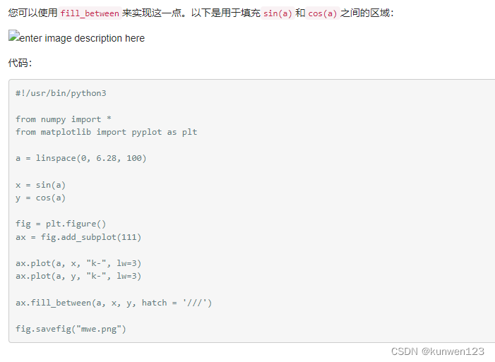
#!/usr/bin/python3

from numpy import *
from matplotlib import pyplot as plt

a = linspace(0, 6.28, 100)

x = sin(a)
y = cos(a)

fig = plt.figure()
ax = fig.add_subplot(111)

ax.plot(a, x, "k-", lw=3)
ax.plot(a, y, "k-", lw=3)

ax.fill_between(a, x, y, hatch = '///')

fig.savefig("mwe.png")

import numpy as np
from matplotlib import pyplot as plt
from sympy import sin


def fun1(x):
    # return x**3-1/x
    return 1/x**2
def numerical_lim(f,x):
    h=1e-4
    return (f(x+h)-f(x))/h
def tangent_line(f,x):
    #d就是调用numerical_diff求得在x点点导数
    d=numerical_lim(f,x)
    # 这里直接y=kx+b求截，简单粗暴，y就是截距
    y=f(x)-d*x
    #使用lambda匿名函数，t是形参，'：'后是要执行的函数表达式
    return lambda t:d*t+y
x=np.arange(0.0,20.0,0.1)
y=fun1(x)
plt.xlabel('x')
plt.ylabel('f(x)')
#把函数作为形参时i，传入实参函数时，只要函数名即可，不用()
tf=tangent_line(fun1,10)
#因为tf返回的是lambda函数，所以要多调一次函数
y2=tf(x)
plt.plot(x,y)
plt.plot(x,y2)
plt.show()

一、生成主窗口（主窗口操作）
window=tkinter.Tk()
#修改框体的名字,也可在创建时使用className参数来命名；
window.title(‘标题名’)
#框体大小可调性，分别表示x,y方向的可变性；1表示可变，0表示不可变；
window.resizable(0,0)
#指定主框体大小；
window.geometry(‘250x150’)
#退出
window.quit()
window.update_idletasks()
#刷新页面
window.update()
#进入消息循环（必需组件）
window.mainloop（）
二、组件的放置和排版（pack grid place）
1、pack组件设置位置属性参数：
after：将组件置于其他组件之后；
before：将组件置于其他组件之前；
ancho： 组件的对齐方式，顶对齐’n’,底对齐’s’,左’w’,右’e’
side： 组件在主窗口的位置，可以为’top’,‘bottom’,‘left’,‘right’（使用时tkinter.TOP,tkinter.LEFT）；
fill：填充方式 (Y,垂直，X，水平，BOTH，水平+垂直），是否在某个方向充满窗口
expand：1可扩展，0不可扩展，代表控件是否会随窗口缩放

2、grid组件使用行列的方法放置组件的位置，参数有：
column: 组件所在的列起始位置；

columnspan: 组件的列宽；跨列数

row： 组件所在的行起始位置；

rowspan：组件的行宽；rowspam=3 跨3行

sticky ： 对齐方式：NSEW（北南东西）上下左右

padx、pady ：x方向间距、y方向间距（padx=5）

3、place组件可以直接使用坐标来放置组件，参数有：
anchor: ： 组件对齐方式；n, ne, e, se, s, sw, w, nw, or center ; （‘n’==N）
x: 组件左上角的x坐标；
y: 组件左上角的y坐标；
relx: 组件左上角相对于窗口的x坐标，应为0-1之间的小数；图形位置相对窗口变化
rely: 组件左上角相对于窗口的y坐标，应为0-1之间的小数；
width: 组件的宽度；
heitht: 组件的高度；
relwidth: 组件相对于窗口的宽度，0-1之间的小数，图形宽度相对窗口变化；
relheight:　 组件相对于窗口的高度，0-1之间的小数；

python notebook控件 python控件位置
https://blog.51cto.com/u_16099218/6370978
pyinstaller深入使用，打包指定模块，打包静态文件
http://www.taodudu.cc/news/show-263117.html?action=onClick

**

python tkinter customtkinter ttkbootstrap

**
值得拥有的五种Python Tkinter界面美化库！

PyInstaller Manual
Python打包：PyInstaller 教程

python代码的几种常见加密方式分享
PyArmor加密Python代码的django工程
github/pyarmor

pyarmor obfuscate --exact foo.py

div 实现 梯形

创建新的干净的python virtualenv 虚拟环境
https://blog.csdn.net/u013203733/article/details/88864886

pyinstaller——添加库路径以解决引用库函数的exe文件无法运行

#外部库位于python文件夹
pyinstaller -F xxx.py -p D:\python\Lib\site-packages
#外部库位于Pycharm工程文件夹
pyinstaller -F xxx.py -p venv\Lib\site-packages

https://www.python100.com/html/0ATV8446SF6J.html