【Python/机器学习/深度学习】学习笔记5——进阶学习Machine-Learning模型与算法应用——机器学习应用案例
局部可解释性:局部解释促进了对单个数据点或分布的一小部分的理解,例如输入记录和其相应预测值的集群,或预测值的十分位数和相应的输入行。局部可解释的模型无关解释(LIME)是一种算法,它提供了一种新颖的技术,以可解释和忠实的方式解释任何预测模型的结果。教程方法是2020年的,我的sklearn是24年最新版的,所以极有可能是新版的sklearn中版本没有了原来的库导致。全局可解释性:全局解释帮助我们理
目录
(1.2) under_sampling RandomUnderSampler
(2.1) over_sampling SMOTETomek
(2.2) over_sampling RandomOverSampler
(3) Penalize Algorithms (Cost-Sensitive Training)
(7) Change Your Performance Metric
第39课 对于已交付(客户流失预警)模型的模型可解释LIME
第37-38课 基于信用卡交易欺诈非均衡数据的处理
https://www.youtube.com/watch?v=TpGCoIHDJAs&list=PLGkfh2EpdoKU3OssXkTl3y7c9tw7jjvHm&index=37
内容:
数据集包含2013年9月欧洲持卡人使用信用卡进行的交易量。该数据集展示了两天内发生的交易,其中有492笔欺诈交易,总共有284,807笔交易。数据集高度不均衡,正类(欺诈)占所有交易的0.172%。
它只包含数值输入变量,这些变量是PCA变换(组成成分分析:PCA的目标是用方差来衡量数据的差异性,并将差异性较大的高维数据投影到低维空间中表示。这允许我们在更低的维度下查看和分析数据,从而可以更方便地进行进一步的数据分析,同时减少了数据的复杂性。)的结果。不幸的是,由于保密问题,我们无法提供原始特征和更多关于数据的背景信息。特征V1、V2、... V28是通过PCA获得的主成分,唯一未使用PCA转换的特征是'Time'和'Amount'。特征'Time'包含每个交易与数据集中的第一个交易之间的经过的秒数。特征'Amount'是交易金额,例如这个特征可以用于示例依赖的成本敏感学习。特征'Class'是响应变量,如果存在欺诈行为,则取值为1,否则为0。
不均衡数据集可以在各种领域中使用:
金融:欺诈检测数据集通常具有约1-2%的欺诈率。广告投放:点击预测数据集也没有很高的点击率。
交通/航空:飞机会坠毁吗?
医疗:患者是否患有癌症?
内容审核:帖子是否包含NSFW内容?(NSFW是一个英文网络用语,“Not Safe For Work”或者“Not Suitable For Work”的缩写,意思就是某个网络内容不适合上班时间浏览。这个词汇经常用在包含成人内容、暴力、冒犯甚至政治内容的网页、视频、照片或音频链接上,作为警告提示用户这些内容可能不适合在工作环境中查看。)
from IPython.display import Image
Image(filename='./Lesson37-dealing imbalance data.png')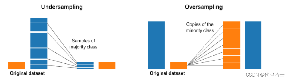
import numpy as np
import pandas as pd
import sklearn
import matplotlib.pyplot as plt
import seaborn as sns
from sklearn.metrics import classification_report,accuracy_score
from sklearn.metrics import confusion_matrix
import warnings
warnings.filterwarnings("ignore")

from sklearn.svm import OneClassSVM
from pylab import rcParams
from sklearn.metrics import precision_score
rcParams['figure.figsize'] = 14, 8
RANDOM_SEED = 42
LABELS = ["Normal", "Fraud"]
data = pd.read_csv('creditcard.csv',sep=',')
data 数据来源:creditcard.csv | Kaggle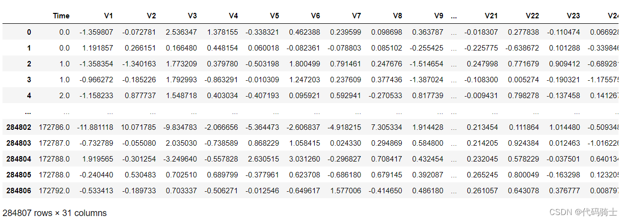

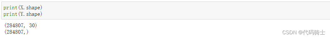
Y = data['Class']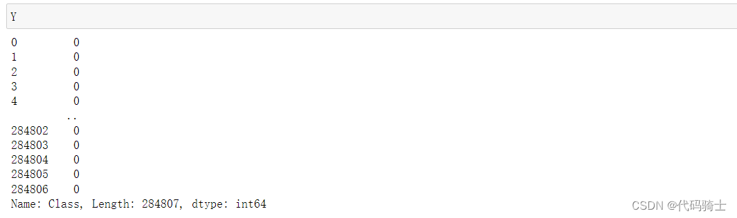
X = data.drop('Class',axis=1,inplace=False)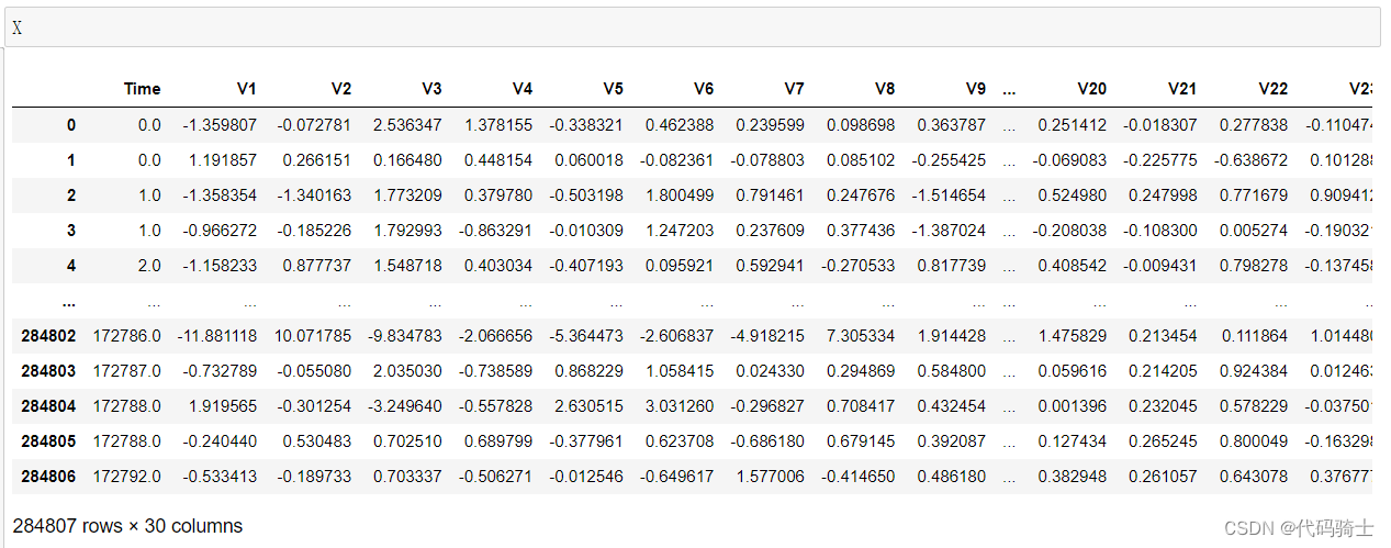
Exploratory Data Analysis
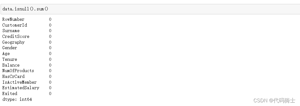
data.isnull().values.any()False
count_classes = pd.value_counts(data['Class'], sort = True)

count_classes.plot(kind = 'bar', rot=0)

plt.title("Transaction Class Distribution")

plt.xticks(range(2), LABELS)

plt.xlabel("Class")

plt.ylabel("Frequency")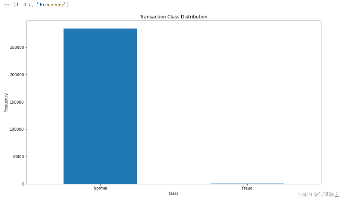
## Get the Fraud and the normal dataset

fraud = data[data['Class']==1]

normal = data[data['Class']==0] 
使用xboost建模。(属于普通建模,并不能合理判断出非均衡数据。意思是做出的分类结果大部分都是正常数据,因为训练集中被诈骗的数据毕竟是少数,要想敏感找出这种数据必须使用udersampling或者oversampling模型算法)
pip install xgboostfrom xgboost import XGBClassifier
from sklearn.model_selection import train_test_split
from sklearn.metrics import accuracy_score
X_train, X_test, y_train, y_test = train_test_split(X, Y, test_size=0.3, random_state=1)
model = XGBClassifier()
model.fit(X_train, y_train)
y_pred = model.predict(X_test)
accuracy = accuracy_score(y_test, y_pred)
print("Accuracy: %.2f%%" % (accuracy * 100.0))Accuracy: 99.95%
这个准确率是区分诈骗和非诈骗两个类别的准确率,我们应该关注的是精确率。实际上这个模型并不能解决我们此次信用卡交易欺诈非均衡数据的处理,这里只是举个反例。
confusion_matrix(y_true=y_test, y_pred=y_pred)array([[85297, 11],
[ 31, 104]], dtype=int64)
precision_score(y_test, y_pred)0.9043478260869565
from matplotlib import pyplot as plt

conf_mat = confusion_matrix(y_true=y_test, y_pred=y_pred)
print('Confusion matrix:\n', conf_mat)

labels = ['Class 0', 'Class 1']
fig = plt.figure()
ax = fig.add_subplot(111)
cax = ax.matshow(conf_mat, cmap=plt.cm.Blues)
fig.colorbar(cax)
ax.set_xticklabels([''] + labels)
ax.set_yticklabels([''] + labels)
plt.xlabel('Predicted')
plt.ylabel('Expected')
plt.show()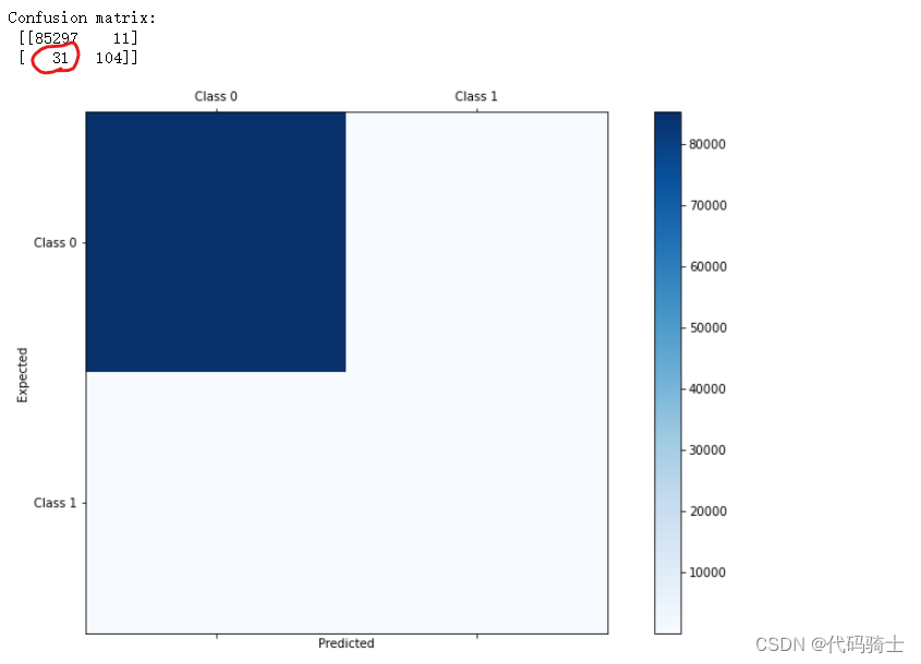
这里有31个诈骗数据没有甄别出来,并不符合我们本次的要求。
(1.1) under_sampling NearMiss
pip install imbalanced-learn库安装失败……(以下是成功例子截图)
#conda install -c conda-forge imbalanced-learn

from imblearn.under_sampling import NearMiss
报错说明:cannot import name '_OneToOneFeatureMixin' from 'sklearn.base' (C:\ProgramData\Anaconda3\lib\site-packages\sklearn\base.py)
教程方法是2020年的,我的sklearn是24年最新版的,所以极有可能是新版的sklearn中版本没有了原来的库导致。——版本不兼容。
解决方法:
1、查阅官方网站的最新使用方法。Getting Started — Version 0.12.0
2、对sklearn降级pip install scikit-learn==0.20
但均为得到有效解决……
from IPython.display import Image
Image(filename='./Lesson37-python-resampling.jpg')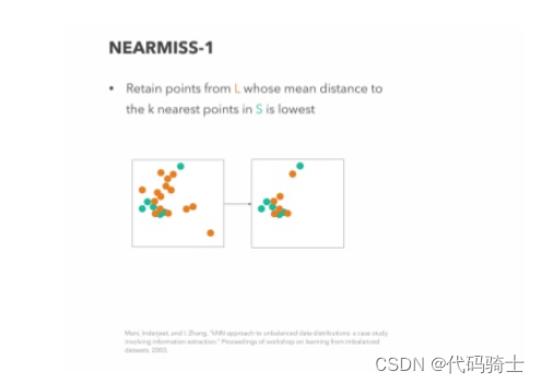
# Implementing Undersampling for Handling Imbalanced
#nm = NearMiss(random_state=42)
nm = NearMiss()
X_res,y_res=nm.fit_sample(X,Y)
from collections import Counter
print('Original dataset shape {}'.format(Counter(Y)))
print('Resampled dataset shape {}'.format(Counter(y_res)))
Original dataset shape Counter({0: 284315, 1: 492})
Resampled dataset shape Counter({0: 492, 1: 492})
X_train, X_test, y_train, y_test = train_test_split(X_res, y_res, test_size=0.3, random_state=1)

model = XGBClassifier()
model.fit(X_train, y_train)
y_pred = model.predict(X_test)

accuracy = accuracy_score(y_test, y_pred)
print("Accuracy: %.2f%%" % (accuracy * 100.0))
Accuracy: 95.27%
confusion_matrix(y_true=y_test, y_pred=y_pred)array([[140, 2],
[ 12, 142]], dtype=int64)
precision_score(y_test, y_pred)0.9861111111111112
使用under_sampling处理非均衡数据,在此模型中仅有12个诈骗数据没有判断出来,精确率达到0.98,得到大幅提高。
(1.2) under_sampling RandomUnderSampler
from IPython.display import Image
Image(filename='./Lesson37-python-resampling-16-638.jpg')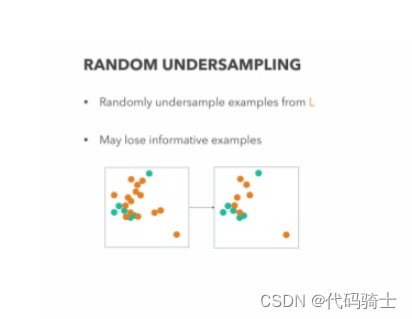
from imblearn.under_sampling import RandomUnderSampler

rus = RandomUnderSampler(random_state=0)
rus.fit(X, Y)
X_res, y_res = rus.fit_sample(X, Y)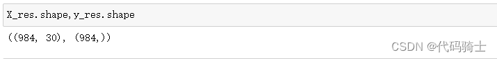
from collections import Counter
print('Original dataset shape {}'.format(Counter(Y)))
print('Resampled dataset shape {}'.format(Counter(y_res)))
Original dataset shape Counter({0: 284315, 1: 492})
Resampled dataset shape Counter({0: 492, 1: 492})
X_train, X_test, y_train, y_test = train_test_split(X_res, y_res, test_size=0.3, random_state=1)

model = XGBClassifier()
model.fit(X_train, y_train)
y_pred = model.predict(X_test)

accuracy = accuracy_score(y_test, y_pred)
print("Accuracy: %.2f%%" % (accuracy * 100.0))
Accuracy: 94.59%
confusion_matrix(y_true=y_test, y_pred=y_pred)array([[139, 3],
[ 13, 141]], dtype=int64)
precision_score(y_test, y_pred)0.9791666666666666
under_sampling
Advantages
It can help improve run time and storage problems by reducing the number of training data samples when the training data set is huge.
Disadvantages
It can discard potentially useful information which could be important for building rule classifiers. The sample chosen by random under sampling may be a biased sample. And it will not be an accurate representative of the population. Thereby, resulting in inaccurate results with the actual test data set.
(2.1) over_sampling SMOTETomek
https://imbalanced-learn.readthedocs.io/en/stable/api.html#module-imblearn.over_sampling
Synthetic Minority Oversampling Technique(SMOTE)
Tomek link:A pair of examples is called a Tomek link if they belong to different classes and are each other's nearest neighbors. Undersampling can be done by removing all tomek links from the dataset
Class to perform over-sampling using SMOTE and cleaning using Tomek links.
Combine over- and under-sampling using SMOTE and Tomek links.
from imblearn.combine import SMOTETomek

# Implementing Oversampling for Handling Imbalanced
smk = SMOTETomek(random_state=42)
X_res,y_res=smk.fit_sample(X,Y)
Image(filename='./Lesson38-oversampling2.png')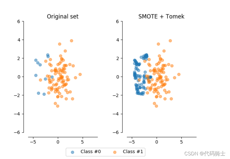

from collections import Counter
print('Original dataset shape {}'.format(Counter(Y)))
print('Resampled dataset shape {}'.format(Counter(y_res)))
Original dataset shape Counter({0: 284315, 1: 492})
Resampled dataset shape Counter({0: 283781, 1: 283781})
X_train, X_test, y_train, y_test = train_test_split(X_res, y_res, test_size=0.3, random_state=1)

model = XGBClassifier()
model.fit(X_train, y_train)
y_pred = model.predict(X_test)

accuracy = accuracy_score(y_test, y_pred)
print("Accuracy: %.2f%%" % (accuracy * 100.0))
Accuracy: 98.73%
confusion_matrix(y_true=y_test, y_pred=y_pred)array([[84746, 547],
[ 1618, 83358]], dtype=int64)
precision_score(y_test, y_pred)0.9934807222453966
(2.2) over_sampling RandomOverSampler
## RandomOverSampler to handle imbalanced data

from imblearn.over_sampling import RandomOverSampler
Image(filename='./Lesson38-oversampling1.png')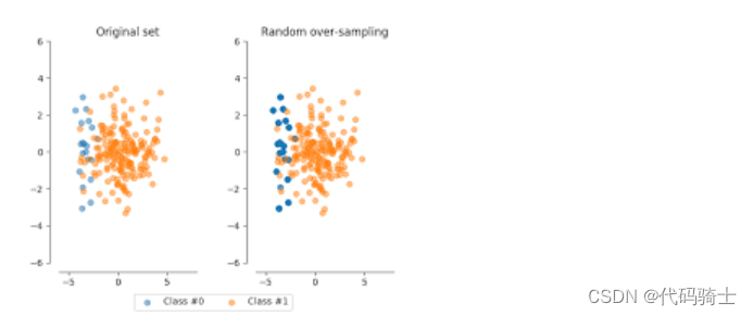
os = RandomOverSampler(random_state=10)X_res, y_res = os.fit_sample(X, Y)X_res.shape,y_res.shape((568630, 30), (568630,))
print('Original dataset shape {}'.format(Counter(Y)))
print('Resampled dataset shape {}'.format(Counter(y_res)))
Original dataset shape Counter({0: 284315, 1: 492})
Resampled dataset shape Counter({0: 284315, 1: 284315})
X_train, X_test, y_train, y_test = train_test_split(X_res, y_res, test_size=0.3, random_state=1)

model = XGBClassifier()
model.fit(X_train, y_train)
y_pred = model.predict(X_test)

accuracy = accuracy_score(y_test, y_pred)
print("Accuracy: %.2f%%" % (accuracy * 100.0))
Accuracy: 99.39%
confusion_matrix(y_true=y_test, y_pred=y_pred)array([[84739, 689],
[ 344, 84817]], dtype=int64)
precision_score(y_test, y_pred)0.9919420859354899
over_sampling
Advantages
Unlike under sampling this method leads to no information loss. Outperforms under sampling
Disadvantages
It increases the likelihood of overfitting since it replicates the minority class events.
(3) Penalize Algorithms (Cost-Sensitive Training)
using penalized learning algorithms that increase the cost of classification mistakes on the minority class
from sklearn.model_selection import train_test_split
from sklearn.preprocessing import StandardScaler
from sklearn.svm import SVC
X_train, X_test, y_train, y_test = train_test_split(X, Y, test_size=0.30, random_state=42)
scaler = StandardScaler()
X_train=scaler.fit_transform(X_train)
X_test=scaler.transform(X_test)
#scaler = StandardScaler()
#Xstan = scaler.fit_transform(X)# Train model
clf_3 = SVC(kernel='linear',
class_weight='balanced', # penalize
probability=True)
clf_3.fit(X_train, y_train)
# Predict on training set
pred_y_3 = clf_3.predict(X_test)(4) Most of the machine learning models provide a parameter called class_weights. For example, in a random forest classifier using, class_weights we can specify a higher weight for the minority class using a dictionary.、
from sklearn.linear_model import LogisticRegression
clf = LogisticRegression(class_weight={0:1,1:10})
(5) from sklearn.utils.class_weight import compute_class_weightclass_weights = compute_class_weight('balanced', np.unique(y), y)
(6) Use Tree-Based Algorithms
. Decision trees often perform well on imbalanced datasets because their hierarchical structure allows them to learn signals from both classes.
In modern applied machine learning, tree ensembles (Random Forests, Gradient Boosted Trees, etc.) almost always outperform singular decision trees, so we'll jump right into those
from sklearn.ensemble import RandomForestClassifier(7) Change Your Performance Metric
For a general-purpose metric for classification, we recommend Area Under ROC Curve (AUROC).
Note: if you got an AUROC of 0.47, it just means you need to invert the predictions because Scikit-Learn is misinterpreting the positive class. AUROC should be >= 0.5.
from sklearn.metrics import roc_auc_score(8) neural network (待续)
其他大佬的操作:
creditcard handling imbalanced dataset | Kaggle
Credit Card Fraud Detection | Kaggle
第39课 对于已交付(客户流失预警)模型的模型可解释LIME
局部可解释的模型无关解释(LIME)是一种算法,它提供了一种新颖的技术,以可解释和忠实的方式解释任何预测模型的结果。它的工作原理是在你想要解释的预测周围局部训练一个可解释的模型。
“为什么我应该相信你?解释任何分类器的预测。”
Improving model interpretability with LIME - The SAS Data Science Blog
定义问题陈述
假设生成
数据探索
预处理
特征工程
模型构建
模型部署
from IPython.display import Image
Image(filename='./Lesson39-LIME3.png')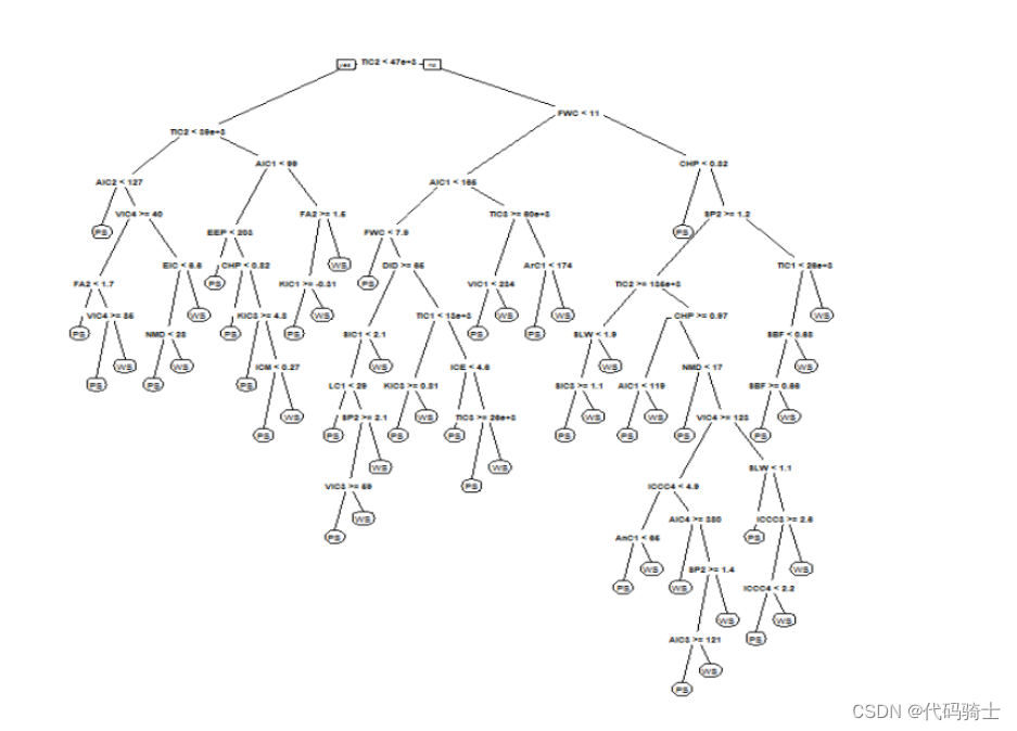
Image(filename='./Lesson39-LIME0.png')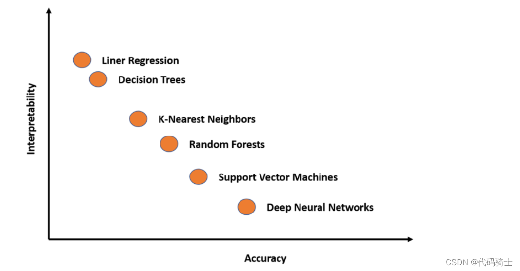
Image(filename='./Lesson39-LIME1.png')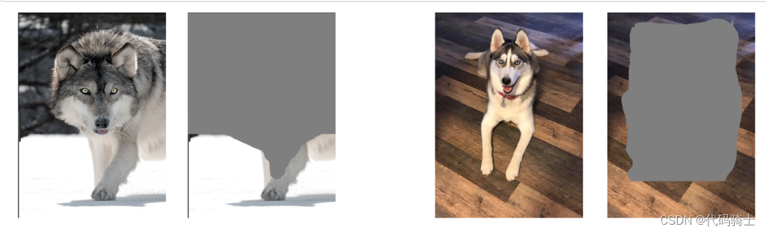
Image(filename='./Lesson39-LIME.png')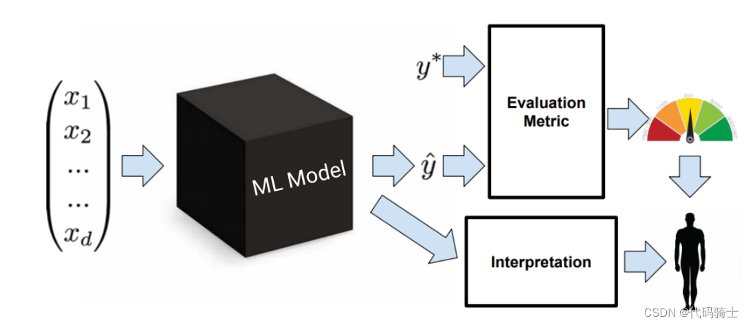
from IPython.display import Image
Image(filename='./Lesson39-.png')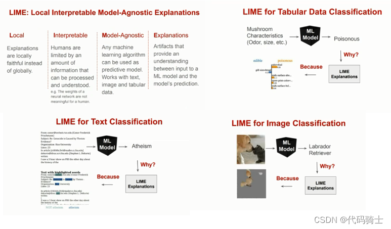
全局可解释性:全局解释帮助我们理解由训练后的响应函数所建模的整个条件分布,但全局解释可能是近似的或基于平均值的。
局部可解释性:局部解释促进了对单个数据点或分布的一小部分的理解,例如输入记录和其相应预测值的集群,或预测值的十分位数和相应的输入行。由于条件分布的小部分更可能是线性的,因此局部解释可能比全局解释更准确。
Image(filename='./Lesson39-LIME2.png')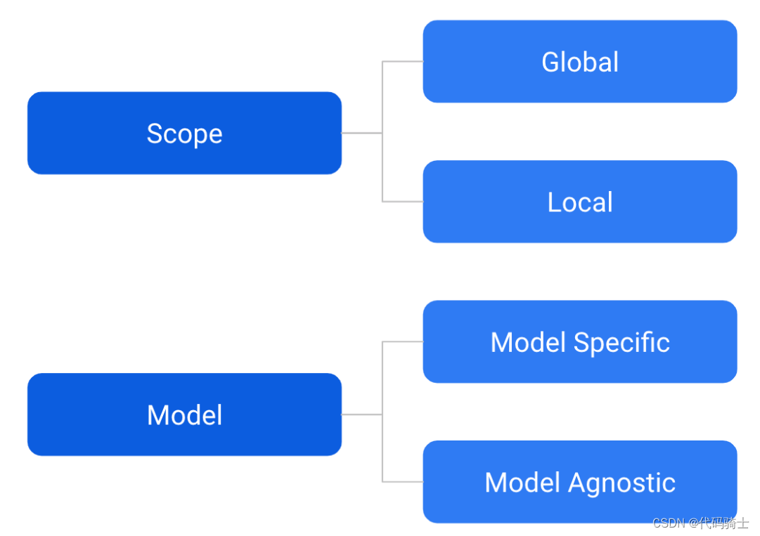
# Part 1 - Data Preprocessing

# Importing the libraries
import numpy as np
import matplotlib.pyplot as plt
import pandas as pd
# Importing the dataset
data = pd.read_csv('Lesson39-Churn_Modelling.csv')
X = data.iloc[:, 3:13]
y = data.iloc[:, 13]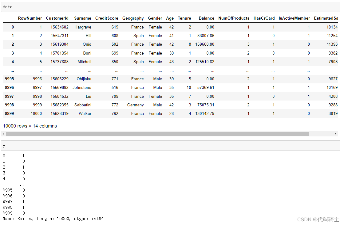
#Create dummy variables
geography=pd.get_dummies(X["Geography"],drop_first=True)
gender=pd.get_dummies(X['Gender'],drop_first=True)
## Concatenate the Data Frames
X=pd.concat([X,geography,gender],axis=1)
## Drop Unnecessary columns
X=X.drop(['Geography','Gender'],axis=1)# Splitting the dataset into the Training set and Test set
from sklearn.model_selection import train_test_split
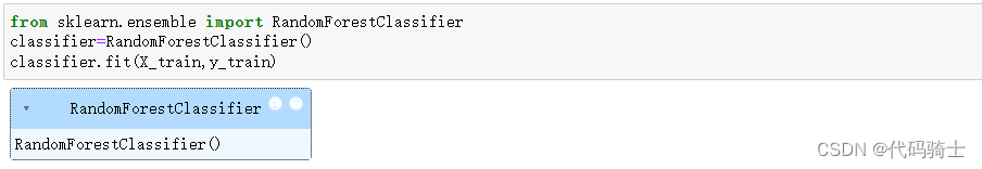
X_train, X_test, y_train, y_test = train_test_split(X, y, test_size = 0.3, random_state = 0)from sklearn.ensemble import RandomForestClassifier
classifier=RandomForestClassifier()
classifier.fit(X_train,y_train)RandomForestClassifier(bootstrap=True, ccp_alpha=0.0, class_weight=None,
criterion='gini', max_depth=None, max_features='auto',
max_leaf_nodes=None, max_samples=None,
min_impurity_decrease=0.0, min_impurity_split=None,
min_samples_leaf=1, min_samples_split=2,
min_weight_fraction_leaf=0.0, n_estimators=100,
n_jobs=None, oob_score=False, random_state=None,
verbose=0, warm_start=False)
X_test.iloc[:, :]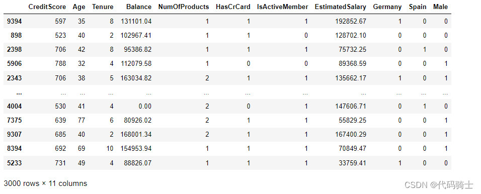
X_test.iloc[[0], :]
X_observation = X_test.iloc[[0], :]

#* RF prediction: {rf_model.predict(X_observation)[0]}

print('prediction: {}'.format(classifier.predict(X_observation)))
prediction: [0]
X_test.iloc[[1],:]
print('prediction: {}'.format(classifier.predict(X_test.iloc[[0],:])))prediction: [0]
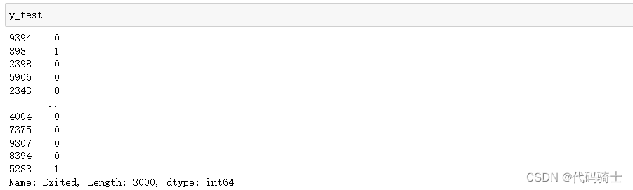
y_pred=classifier.predict(X_test)
#Import scikit-learn metrics module for accuracy calculation
from sklearn import metrics

# Model Accuracy, how often is the classifier correct?
print("Accuracy:",metrics.accuracy_score(y_test, y_pred))
Accuracy: 0.8666666666666667
# Extract single tree
estimator = classifier.estimators_[10]

from sklearn.tree import export_graphviz
# Export as dot file
export_graphviz(estimator,
                out_file='tree.dot',
                feature_names = X_train.columns,
                class_names = y_train.name,
                rounded = True, proportion = True,
                precision = 2, filled = True)
#export_graphviz(estimator, feature_names = X_train.columns)
!dot -Tpng tree.dot -o tree_limited.png -Gdpi=600
# Display in jupyter notebook
from IPython.display import Image
Image(filename = 'tree_limited.png')
import pickle
pickle.dump(classifier, open("classifier.pkl", 'wb')) 
classifier1=pd.read_pickle('classifier.pkl')!pip install limeCollecting lime Downloading lime-0.2.0.1.tar.gz (275 kB) Requirement already satisfied: matplotlib in c:\users\raymond\anaconda3\lib\site-packages (from lime) (3.3.2) Requirement already satisfied: numpy in c:\users\raymond\anaconda3\lib\site-packages (from lime) (1.19.2) Requirement already satisfied: scipy in c:\users\raymond\anaconda3\lib\site-packages (from lime) (1.5.2) Requirement already satisfied: tqdm in c:\users\raymond\anaconda3\lib\site-packages (from lime) (4.51.0) Requirement already satisfied: scikit-learn>=0.18 in c:\users\raymond\anaconda3\lib\site-packages (from lime) (0.22.1) Requirement already satisfied: scikit-image>=0.12 in c:\users\raymond\anaconda3\lib\site-packages (from lime) (0.17.2) Requirement already satisfied: kiwisolver>=1.0.1 in c:\users\raymond\anaconda3\lib\site-packages (from matplotlib->lime) (1.3.0) Requirement already satisfied: pillow>=6.2.0 in c:\users\raymond\anaconda3\lib\site-packages (from matplotlib->lime) (8.0.1) Requirement already satisfied: python-dateutil>=2.1 in c:\users\raymond\anaconda3\lib\site-packages (from matplotlib->lime) (2.8.1) Requirement already satisfied: certifi>=2020.06.20 in c:\users\raymond\anaconda3\lib\site-packages (from matplotlib->lime) (2020.12.5) Requirement already satisfied: cycler>=0.10 in c:\users\raymond\anaconda3\lib\site-packages (from matplotlib->lime) (0.10.0) Requirement already satisfied: pyparsing!=2.0.4,!=2.1.2,!=2.1.6,>=2.0.3 in c:\users\raymond\anaconda3\lib\site-packages (from matplotlib->lime) (2.4.7) Requirement already satisfied: joblib>=0.11 in c:\users\raymond\anaconda3\lib\site-packages (from scikit-learn>=0.18->lime) (0.17.0) Requirement already satisfied: networkx>=2.0 in c:\users\raymond\anaconda3\lib\site-packages (from scikit-image>=0.12->lime) (2.5) Requirement already satisfied: imageio>=2.3.0 in c:\users\raymond\anaconda3\lib\site-packages (from scikit-image>=0.12->lime) (2.9.0) Requirement already satisfied: tifffile>=2019.7.26 in c:\users\raymond\anaconda3\lib\site-packages (from scikit-image>=0.12->lime) (2020.10.1) Requirement already satisfied: PyWavelets>=1.1.1 in c:\users\raymond\anaconda3\lib\site-packages (from scikit-image>=0.12->lime) (1.1.1) Requirement already satisfied: six>=1.5 in c:\users\raymond\anaconda3\lib\site-packages (from python-dateutil>=2.1->matplotlib->lime) (1.15.0) Requirement already satisfied: decorator>=4.3.0 in c:\users\raymond\anaconda3\lib\site-packages (from networkx>=2.0->scikit-image>=0.12->lime) (4.4.2) Building wheels for collected packages: lime Building wheel for lime (setup.py): started Building wheel for lime (setup.py): finished with status 'done' Created wheel for lime: filename=lime-0.2.0.1-py3-none-any.whl size=283850 sha256=3852cf2ed5851927515ab1e4e1dda113797c6599b3ab2d0da94261975dc551b7 Stored in directory: c:\users\raymond\appdata\local\pip\cache\wheels\ca\cb\e5\ac701e12d365a08917bf4c6171c0961bc880a8181359c66aa7 Successfully built lime Installing collected packages: lime Successfully installed lime-0.2.0.1
import lime
from lime import lime_tabular

interpretor = lime_tabular.LimeTabularExplainer(
    training_data=np.array(X_train),
    feature_names=X_train.columns,
    mode='classification'
)
X_test.iloc[[88],:]
print('prediction: {}'.format(classifier1.predict(X_test.iloc[[88],:])))prediction: [1]
X_test.iloc[88]CreditScore 756.00 Age 39.00 Tenure 3.00 Balance 100717.85 NumOfProducts 3.00 HasCrCard 1.00 IsActiveMember 1.00 EstimatedSalary 73406.04 Germany 1.00 Spain 0.00 Male 0.00 Name: 1096, dtype: float64
# feature importance of the random forest model
feature_importance = pd.DataFrame()
feature_importance['variable'] = X_train.columns
feature_importance['importance'] = classifier1.feature_importances_

# feature_importance values in descending order
feature_importance.sort_values(by='importance', ascending=False).head(10)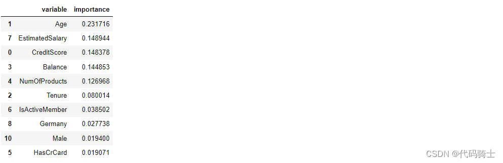
exp = interpretor.explain_instance(
    data_row=X_test.iloc[88], ##new data
    predict_fn=classifier1.predict_proba
)

exp.show_in_notebook(show_table=True)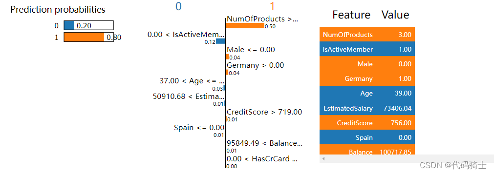
exp.as_pyplot_figure()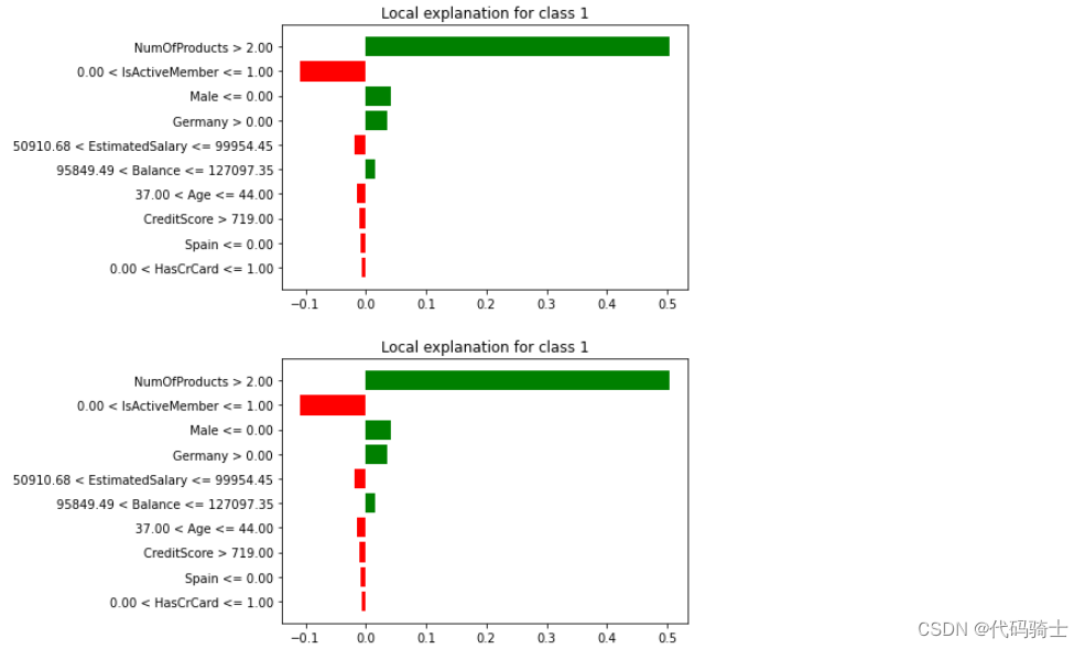
exp = interpretor.explain_instance(
    data_row=X_test.iloc[2], ##new data
    predict_fn=classifier1.predict_proba,
    num_features=10
)X_test.iloc[2]CreditScore 706.00 Age 42.00 Tenure 8.00 Balance 95386.82 NumOfProducts 1.00 HasCrCard 1.00 IsActiveMember 1.00 EstimatedSalary 75732.25 Germany 0.00 Spain 1.00 Male 0.00 Name: 2398, dtype: float64
exp.show_in_notebook(show_table=True,show_all=False)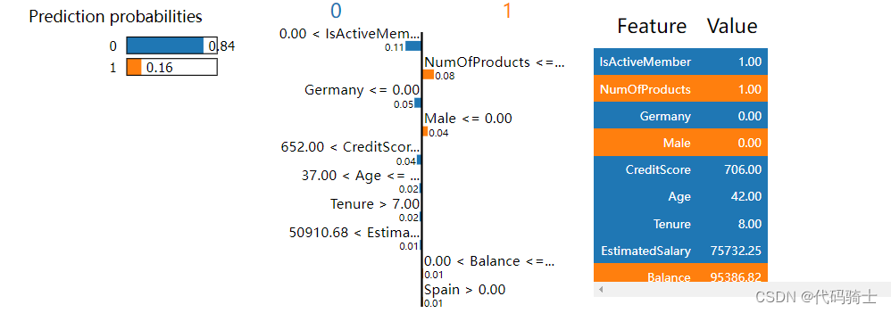
exp.as_pyplot_figure()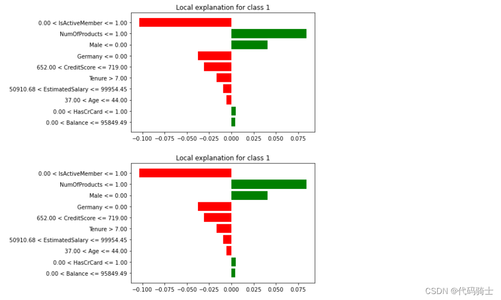
exp.as_list()[('0.00 < IsActiveMember <= 1.00', -0.1034779933529071),
('NumOfProducts <= 1.00', 0.08432655331131134),
('Male <= 0.00', 0.04093426823831788),
('Germany <= 0.00', -0.03770485115176004),
('652.00 < CreditScore <= 719.00', -0.03061889433199798),
('Tenure > 7.00', -0.016548478267618315),
('50910.68 < EstimatedSalary <= 99954.45', -0.00954760526017956),
('37.00 < Age <= 44.00', -0.005501744385790516),
('0.00 < HasCrCard <= 1.00', 0.004924918916634485),
('0.00 < Balance <= 95849.49', 0.004215444410328281)]
腾讯云面向开发者汇聚海量精品云计算使用和开发经验,营造开放的云计算技术生态圈。
更多推荐
 12
12 0
0- 0


 已为社区贡献7条内容

所有评论(0)