[深度学习]YOLOV5预处理和后处理,源码分析
关于模型输出的说明(1, 25200, 85):👇⭐25200:每个batch的检测框数量⭐85:每个检测框包含信息[x, y, w, h, 置信度, coco_class0_score, coco_class1_score, …, …, coco_class79_score]conf_thres = 0.001 # 置信度筛选阈值max_wh = 7680 # 最大允许的检测框高宽iou_th
2024.10.7.补充
现在yolo各个版本可以统一使用Ultralytics包进行训练,预处理的关键代码入口位置有变动,我的这篇博客有重新定位代码位置,分析了yolov10的train和val阶段各自的预处理代码入口。
前言
推理性能与哪些方面有关?
- 模型量化(FP32、FP16、INT8、INT4、Bool等等)
- 算子支持(Pool、BatchNorm等等)
- 预处理和后处理(本文的关注点)
分析的代码是------>下面图中<------这个位置的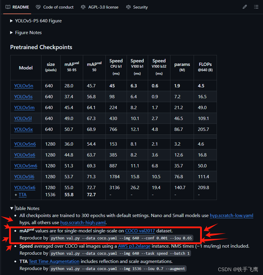
yolov5预处理
1 关键代码在yolov5源码中的位置:👇
⭐解释👇:在val.py中每次加载图片都会调用一次def __getitem __(self, index)。
yolov5/utils/dataloaders.py---------->第764行---------->def __getitem __(self, index)
⭐解释👇:在def __getitem __(self, index)内会调用def load_image(im_path, img_size)来读取图片。
yolov5/utils/dataloaders.py---------->第841行---------->def load_image(im_path, img_size)
⭐解释👇:在def load_image(im_path, img_size)之后,会调用def letterbox对图片预处理:resize---->padding---->转RGB---->转(3,640,640),最后回到val.py中进行归一化。
yolov5/utils/augmentations.py---------->第121行---------->def letterbox(im, new_shape=(640, 640), color=(114, 114, 114), auto=True, scaleFill=False, scaleup=True, stride=32)
2 下面是演示预处理主要流程
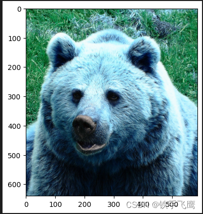
2.1 读取图片
import cv2
import numpy as np
import torch, torchvision
import math
import matplotlib.pyplot as plt

original_im = cv2.imread('/home/f/mycode/datasets/coco/images/val2017/000000000285.jpg')  # BGR
im = original_im
img_size = 640  # 假设模型输入图片要求640*640

# 如果在 Jupyter Notebook 中运行,则使用 matplotlib 显示图像
plt.imshow(im)
plt.show()
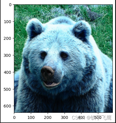
2.2 resize
h0, w0 = im.shape[:2]  # original dimensions
r = img_size / max(h0, w0)  # ratio
if r != 1:  # if sizes are not equal
	interp = cv2.INTER_LINEAR if r > 1 else cv2.INTER_AREA  # 上采样 or 下采样
	im = cv2.resize(im, (math.ceil(w0 * r), math.ceil(h0 * r)), interpolation=interp)

h1, w1 = im.shape[:2]  # resize dimensions

# 如果在 Jupyter Notebook 中运行,则使用 matplotlib 显示图像
plt.imshow(im)
plt.show()
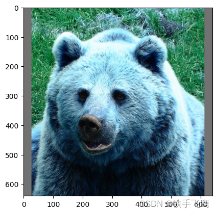
2.3 填充
dw = (img_size - w1) / 2 # 要填充的宽度的一半
dh = (img_size - h0) / 2 # 要填充的高度的一半
top, bottom = int(round(dh - 0.1)), int(round(dh + 0.1))
left, right = int(round(dw - 0.1)), int(round(dw + 0.1))
color = (114, 114, 114) #padding颜色
im = cv2.copyMakeBorder(im, top, bottom, left, right, cv2.BORDER_CONSTANT, value=color)  # add border

# 如果在 Jupyter Notebook 中运行,则使用 matplotlib 显示图像
plt.imshow(im)
plt.show()
2.4 BGR to RGB、(640, 640, 3) 转 (3, 640, 640)
# Convert image to PyTorch tensor and transpose
im = im.transpose((2, 0, 1))[::-1]  # HWC to CHW, BGR to RGB
im = np.ascontiguousarray(im)

print(im.shape) # (3, 640, 640)
2.5 归一化,(3, 640, 640) 转 (1, 3, 640, 640)
input_image = np.expand_dims(im, axis=0).astype(np.float32) / 255.0
print(input_image.shape) # (1, 3, 640, 640)
print(input_image.dtype) # float32
推理一张预处理后的图片获得一次模型输出,方便后处理演示
import openvino as ov

# 模型路径
ir_filename = "/home/f/mycode/mAP_fx/coco/annotations/yolov5n_openvino_model/yolov5n.xml"
# Create OpenVINO Core
core = ov.Core()
# 读取模型
model = core.read_model(model=ir_filename, weights=ir_filename.replace(".xml", ".bin"))
# 加载模型到GPU
compiled_model = core.compile_model(model=model, device_name="GPU")
# 推理
preds = compiled_model(input_image)[0]
print(preds.shape) # (1, 25200, 85)
yolov5后处理
1 关键代码在yolov5源码中的位置:👇
⭐解释👇:从模型输出---->NMS,大部分后处理过程都在这
yolov5/utils/general.py---------->第1005行---------->def non_max_suppression
⭐解释👇:模型推理输出的检测框坐标映射回原图像尺寸坐标
yolov5/utils/general.py---------->第948行---------->def scale_boxes
2 下面是演示后处理主要流程
2.1 获取模型输出的基本信息,定义一些变量
关于模型输出的说明(1, 25200, 85):👇
⭐1: batch
⭐25200: 每个batch的检测框数量
⭐85: 每个检测框包含信息[x, y, w, h, 置信度, coco_class0_score, coco_class1_score, …, …, coco_class79_score]
bs = preds.shape[0]      # batch size
nc = preds.shape[2] - 5  # number of classes
conf_thres = 0.001       # 置信度筛选阈值
max_wh = 7680            # 最大允许的检测框高宽
iou_thres = 0.65         # NMS交并比
max_nms = 30000          # 最多允许30000个框进入NMS
max_det=300              # 保留NMS后的前300个框
output = [np.zeros((0, 6))] * bs# 用来装NMS后的前300个框
2.2 定义几个检测框坐标转换函数
# (左上角坐标,右下角坐标)转 (检测框中心坐标,检测框宽高)
def xyxy2xywh(x):
    """Convert nx4 boxes from [x1, y1, x2, y2] to [x, y, w, h] where xy1=top-left, xy2=bottom-right."""
    y = x.clone() if isinstance(x, torch.Tensor) else np.copy(x)
    y[..., 0] = (x[..., 0] + x[..., 2]) / 2  # x center
    y[..., 1] = (x[..., 1] + x[..., 3]) / 2  # y center
    y[..., 2] = x[..., 2] - x[..., 0]  # width
    y[..., 3] = x[..., 3] - x[..., 1]  # height
    return y

# (检测框中心坐标,检测框宽高)转(左上角坐标,右下角坐标)
def xywh2xyxy(x):
    """Convert nx4 boxes from [x, y, w, h] to [x1, y1, x2, y2] where xy1=top-left, xy2=bottom-right."""
    y = np.copy(x)
    y[..., 0] = x[..., 0] - x[..., 2] / 2  # top left x
    y[..., 1] = x[..., 1] - x[..., 3] / 2  # top left y
    y[..., 2] = x[..., 0] + x[..., 2] / 2  # bottom right x
    y[..., 3] = x[..., 1] + x[..., 3] / 2  # bottom right y
    return y
2.3 NMS之前要对模型输出进行的操作
yolov5的val.py使用的NMS来自torchvision.ops.nms
xc = preds[..., 4] > conf_thres  # 用来筛选出置信度 > 0.001的检测框
print('⭐xc.shape', xc.shape)
print('⭐xc', xc)

# 这个for循环是为了遍历每个batch,此时演示的batch=1,所以只会循环一次,循环内x.shape=(25200,85)
for xi, x in enumerate(preds):
    # xi = 当前遍历的batch_index, x = 筛选置信度大于0.001的检测框
    x = x[xc[xi]]
    # 所有coco_class_score* 乘 confidence
    x[:, 5:] *= x[:, 4:5]
    # 检测框坐标转换,(检测框中心坐标,检测框宽高)转(左上角坐标,右下角坐标)
    box = xywh2xyxy(x[:, :4])
    # mask暂时没什么用
    mask = x[:, 85:]
    # i = 满足要求的检测框index, j = 满足要求的coco类别index
    i, j = np.where(x[:, 5:] > conf_thres)
    # 拼接矩阵,最后x矩阵一共6列, x = (0:4检测框坐标, 4coco_class_score, 5coco_class, mask是空不会占一列)
    x = np.concatenate((box[i], x[i, 5 + j, None], j[:, None].astype(float), mask[i]), axis=1)
    print('⭐x.shape', x.shape)
    # x矩阵根据第五列进行降序排序
    sorted_indices = np.argsort(x[:, 4])[::-1]
    # 保留x排序后的前30000行
    x = x[sorted_indices[:max_nms]]
    # 🤓c的作用意义不明
    c = x[:, 5:6] * max_wh  # classes
    # boxes (offset by class), scores
    boxes, scores = x[:, :4] + c, x[:, 4]
    boxes_tensor = torch.from_numpy(boxes)
    scores_tensor = torch.from_numpy(scores)
    # NMS
    i = torchvision.ops.nms(boxes_tensor, scores_tensor, iou_thres)
    # 保留前300个框
    i = i[:max_det]  # limit detections
    output[xi] = x[i]
    output = np.array(output)
    print('⭐output.shape', output.shape)
    print('⭐output👇\n', output)
打印输出👇
⭐xc.shape (1, 25200)
⭐xc [[False False False … False False False]]
⭐x.shape (291, 6)
⭐output.shape (1, 29, 6)
⭐output👇
[[[4.57500000e+01 9.50000000e+01 6.15750000e+02 6.69500000e+02
4.59377289e-01 2.10000000e+01]
[3.72500000e+01 8.97500000e+01 5.90750000e+02 6.74750000e+02
5.60317039e-02 2.00000000e+01]
[4.57500000e+01 9.50000000e+01 6.15750000e+02 6.69500000e+02
4.40301895e-02 1.60000000e+01]
[4.57500000e+01 9.50000000e+01 6.15750000e+02 6.69500000e+02
3.26796770e-02 1.90000000e+01]
[3.72500000e+01 8.97500000e+01 5.90750000e+02 6.74750000e+02
1.48500055e-02 2.30000000e+01]
[4.57500000e+01 9.50000000e+01 6.15750000e+02 6.69500000e+02
9.98681784e-03 1.80000000e+01]
[3.85000000e+01 3.49375000e+02 6.15000000e+02 6.40625000e+02
9.74352658e-03 2.10000000e+01]
[2.62500000e+01 9.32500000e+01 3.21750000e+02 6.45750000e+02
8.31713900e-03 2.10000000e+01]
[4.57500000e+01 9.50000000e+01 6.15750000e+02 6.69500000e+02
8.24749470e-03 1.50000000e+01]
[2.37875000e+02 1.00500000e+02 6.13125000e+02 6.51500000e+02
6.58459961e-03 2.10000000e+01]
…
[5.67500000e+01 6.11875000e+01 5.78250000e+02 2.92312500e+02
1.16157532e-03 2.10000000e+01]
[5.82500000e+01 6.65625000e+01 5.70750000e+02 1.96187500e+02
1.13130547e-03 1.80000000e+01]]]
2.4 检测框的坐标映射,COCO数据集类别映射
几点说明:
⭐检测框坐标映射: 从640*640图像的检测框坐标映射回原图像size坐标
⭐COCO数据集类别映射: COCO数据集的instances_val2017.json中, 类别是不连续的从1-90, 但实际上仍然是只有80个类别,如下图所示👇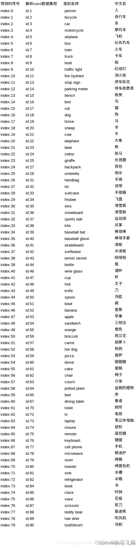
# 因为本例子中,batch=1, 所以output的第一个维度可以不要
print('压缩维度前的output.shape', output.shape)
output = np.squeeze(output, axis=0)
print('压缩维度后的output.shape', output.shape)

# 坐标映射👇
# dw 和 dh 就是预处理时候填充的宽度和高度
output[..., [0, 2]] -= dw  # x padding
output[..., [1, 3]] -= dh  # y padding
# 这里的r,就是预处理时候的r,图像缩放比例
output[..., :4] /= r
# 防止检测框坐标超出图像的范围
output[..., [0, 2]] = output[..., [0, 2]].clip(0, w0)  # x1, x2
output[..., [1, 3]] = output[..., [1, 3]].clip(0, h0)  # y1, y2

# 类别映射👇
# 映射列表
def coco80_to_coco91_class():
    """
    Converts COCO 80-class index to COCO 91-class index used in the paper.

    Reference: https://tech.amikelive.com/node-718/what-object-categories-labels-are-in-coco-dataset/
    """
    # a = np.loadtxt('data/coco.names', dtype='str', delimiter='\n')
    # b = np.loadtxt('data/coco_paper.names', dtype='str', delimiter='\n')
    # x1 = [list(a[i] == b).index(True) + 1 for i in range(80)]  # darknet to coco
    # x2 = [list(b[i] == a).index(True) if any(b[i] == a) else None for i in range(91)]  # coco to darknet
    return [
        1,
        2,
        3,
        4,
        5,
        6,
        7,
        8,
        9,
        10,
        11,
        13,
        14,
        15,
        16,
        17,
        18,
        19,
        20,
        21,
        22,
        23,
        24,
        25,
        27,
        28,
        31,
        32,
        33,
        34,
        35,
        36,
        37,
        38,
        39,
        40,
        41,
        42,
        43,
        44,
        46,
        47,
        48,
        49,
        50,
        51,
        52,
        53,
        54,
        55,
        56,
        57,
        58,
        59,
        60,
        61,
        62,
        63,
        64,
        65,
        67,
        70,
        72,
        73,
        74,
        75,
        76,
        77,
        78,
        79,
        80,
        81,
        82,
        84,
        85,
        86,
        87,
        88,
        89,
        90,
    ]
# 创建一个表
class_map = np.array(coco80_to_coco91_class())
# class_index留着后面画框用
class_index = output[:, 5]
class_index = class_index.astype(int)
# 映射
output[:, 5] = class_map[output[:, 5].astype(int)]
# 最后把检测框坐标(左上角,右下角)转(左上角,宽高)
box = xyxy2xywh(output[:, :4])  # xywh
box[:, :2] -= box[:, 2:] / 2  # xy center to top-left corner
output[:, :4] = box

# 🏁🏁🏁至此,output的内容和yolov5的val.py脚本的后处理结果一致🏁🏁🏁
# 可以在CLI用val.py运行一次:val.py --weights yolov5n_openvino_model --batch-size 1 --data coco.yaml --img 640 --conf 0.001 --iou 0.65
# 在yolov5/runs/val/exp/yolov5n_openvino_model_predictions.json中查找"image_id": 285可以对比output结果
print(output)
打印输出👇
压缩维度前的output.shape (1, 29, 6)
压缩维度后的output.shape (29, 6)
[[1.87500000e+01 9.50000000e+01 5.67250000e+02 5.45000000e+02
4.59377289e-01 2.30000000e+01]
[1.02500000e+01 8.97500000e+01 5.53500000e+02 5.50250000e+02
5.60317039e-02 2.20000000e+01]
[1.87500000e+01 9.50000000e+01 5.67250000e+02 5.45000000e+02
4.40301895e-02 1.80000000e+01]
[1.87500000e+01 9.50000000e+01 5.67250000e+02 5.45000000e+02
3.26796770e-02 2.10000000e+01]
[1.02500000e+01 8.97500000e+01 5.53500000e+02 5.50250000e+02
1.48500055e-02 2.50000000e+01]
[1.87500000e+01 9.50000000e+01 5.67250000e+02 5.45000000e+02
9.98681784e-03 2.00000000e+01]
[1.15000000e+01 3.49375000e+02 5.74500000e+02 2.90625000e+02
9.74352658e-03 2.30000000e+01]
[0.00000000e+00 9.32500000e+01 2.94750000e+02 5.46750000e+02
8.31713900e-03 2.30000000e+01]
[1.87500000e+01 9.50000000e+01 5.67250000e+02 5.45000000e+02
8.24749470e-03 1.70000000e+01]
[2.10875000e+02 1.00500000e+02 3.75125000e+02 5.39500000e+02
6.58459961e-03 2.30000000e+01]
[1.02500000e+01 8.97500000e+01 5.53500000e+02 5.50250000e+02
4.59467992e-03 8.80000000e+01]
[1.95000000e+01 5.61250000e+01 5.24000000e+02 4.64250000e+02
…
[2.97500000e+01 6.11875000e+01 5.21500000e+02 2.31125000e+02
1.16157532e-03 2.30000000e+01]
[3.12500000e+01 6.65625000e+01 5.12500000e+02 1.29625000e+02
1.13130547e-03 2.00000000e+01]]
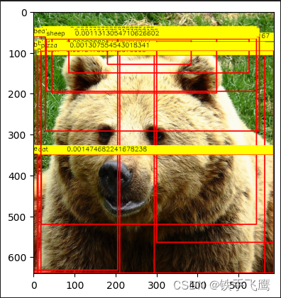
2.5 在原图上画框
# COCO dataset labels
class_names = [
    "person", "bicycle", "car", "motorcycle", "airplane",
    "bus", "train", "truck", "boat", "traffic light",
    "fire hydrant", "stop sign", "parking meter", "bench", "bird",
    "cat", "dog", "horse", "sheep", "cow",
    "elephant", "bear", "zebra", "giraffe", "backpack",
    "umbrella", "handbag", "tie", "suitcase", "frisbee",
    "skis", "snowboard", "sports ball", "kite", "baseball bat",
    "baseball glove", "skateboard", "surfboard", "tennis racket", "bottle",
    "wine glass", "cup", "fork", "knife", "spoon",
    "bowl", "banana", "apple", "sandwich", "orange",
    "broccoli", "carrot", "hot dog", "pizza", "donut",
    "cake", "chair", "couch", "potted plant", "bed",
    "dining table", "toilet", "tv", "laptop", "mouse",
    "remote", "keyboard", "cell phone", "microwave", "oven",
    "toaster", "sink", "refrigerator", "book", "clock",
    "vase", "scissors", "teddy bear", "hair drier", "toothbrush"
]

# 遍历每个框,画框
for object, index in zip(output, class_index):
    x, y, width, height = map(int, object[:4])
    score = str(object[4])
    cv2.rectangle(original_im, (x, y), (x + width, y + height), (0, 0, 255), 2)
    cv2.rectangle(original_im, (x, y - 20), (x + width, y), (0, 255, 255), -1)
    cv2.putText(original_im, class_names[index], (x, y - 8), cv2.FONT_HERSHEY_SIMPLEX, 0.5, (0, 0, 0))
    cv2.putText(original_im, score, (x + 70, y - 8), cv2.FONT_HERSHEY_SIMPLEX, 0.5, (0, 0, 0))

# 如果在 Jupyter Notebook 中运行,则使用 matplotlib 显示图像
plt.imshow(cv2.cvtColor(original_im, cv2.COLOR_BGR2RGB))
plt.show()

腾讯云面向开发者汇聚海量精品云计算使用和开发经验,营造开放的云计算技术生态圈。
更多推荐
 29
29 0
0- 0


 已为社区贡献3条内容

所有评论(0)