Python深度学习--深度学习入门-TensorFlow入门
TensorFlow中的常量 变量 以及 基于TensorFlow实现线性回归与逻辑回归
2. TensorFlow入门
1. 基础API使用
TensorFlow中定义的数据叫做Tensor(张量), Tensor又分为常量和变量.
1.1 常量的定义和使用
常量一旦定义值不能改变.
使用tf.constant定义常量
t = tf.constant([[1., 2., 3.], [4., 5., 6.]])

# 可以像numpy的ndarray一样使用tensor
print(t)
print(t[:, 1:])
print(t[..., 1]) # 或t[:, 1]
输出:
tf.Tensor(
[[1. 2. 3.]
 [4. 5. 6.]], shape=(2, 3), dtype=float32)
tf.Tensor(
[[2. 3.]
 [5. 6.]], shape=(2, 2), dtype=float32)
tf.Tensor([2. 5.], shape=(2,), dtype=float32)
常量的操作:
print(t+10) # 每个元素都加10
print(tf.square(t)) # 每个元素都做平方
print(t @ tf.transpose(t)) # @表示矩阵的点乘
输出:
tf.Tensor(
[[11. 12. 13.]
 [14. 15. 16.]], shape=(2, 3), dtype=float32)
tf.Tensor(
[[ 1.  4.  9.]
 [16. 25. 36.]], shape=(2, 3), dtype=float32)
tf.Tensor(
[[14. 32.]
 [32. 77.]], shape=(2, 2), dtype=float32)
常量tensor和numpy中的ndarray的转化:
# .numpy()可以把tensor转化为ndarray
print(t.numpy())
print(np.square(t))
np_t = np.array([[1., 2., 3.], [4., 5., 6.]])
# 直接使用ndarray生成一个tensor
print(tf.constant(np_t))
输出:
[[1. 2. 3.]
 [4. 5. 6.]]
[[ 1.  4.  9.]
 [16. 25. 36.]]
tf.Tensor(
[[1. 2. 3.]
 [4. 5. 6.]], shape=(2, 3), dtype=float64)
生成标量:
# scalar
t = tf.constant(2.718)
print(t.numpy())
print(t.shape)
输出:
2.718
()
使用字符串
# strings
t = tf.constant("cafe")
print(t)
print(tf.strings.length(t)) # 获取字符串的长度
print(tf.strings.length(t, unit="UTF8_CHAR")) # 获取utf8编码的长度
print(tf.strings.unicode_decode(t, "UTF8")) # 把字符串转化为utf8编码
输出:
tf.Tensor(b'cafe', shape=(), dtype=string)
tf.Tensor(4, shape=(), dtype=int32)
tf.Tensor(4, shape=(), dtype=int32)
tf.Tensor([ 99  97 102 101], shape=(4,), dtype=int32)
使用字符串数组
# string array
t = tf.constant(["cafe", "coffee", "咖啡"])
print(tf.strings.length(t, unit="UTF8_CHAR"))
r = tf.strings.unicode_decode(t, "UTF8")
print(r)
输出:
tf.Tensor([4 6 2], shape=(3,), dtype=int32)
<tf.RaggedTensor [[99, 97, 102, 101], [99, 111, 102, 102, 101, 101], [21654, 21857]]>
ragged tensor 不整齐的tensor, 上面的tensor每个字符串长度不一致.
创建ragged tensor
r = tf.ragged.constant([[11, 12], [21, 22, 23], [], [41]])
# index op
print(r)
print(r[1])
# 左闭右开
print(r[1:2])
输出:
<tf.RaggedTensor [[11, 12], [21, 22, 23], [], [41]]>
tf.Tensor([21 22 23], shape=(3,), dtype=int32)
<tf.RaggedTensor [[21, 22, 23]]>
ragged tensor的操作:
r2 = tf.ragged.constant([[51, 52], [], [71]])
# 拼接操作, axis=0按行拼接. 如果按列拼接会报错. 因为行数不一致.
print(tf.concat([r, r2], axis = 0))
输出:
<tf.RaggedTensor [[11, 12], [21, 22, 23], [], [41], [51, 52], [], [71]]>
按列拼接:
r3 = tf.ragged.constant([[13, 14], [15], [], [42, 43]])
print(tf.concat([r, r3], axis = 1))
输出:
<tf.RaggedTensor [[11, 12, 13, 14], [21, 22, 23, 15], [], [41, 42, 43]]>
把ragged tensor转化为普通tensor
# 缺元素的地方会补0, 0在正常元素的后面.
print(r.to_tensor())
输出:
tf.Tensor(
[[11 12  0]
 [21 22 23]
 [ 0  0  0]
 [41  0  0]], shape=(4, 3), dtype=int32)
sparse tensor 稀疏tensor, tensor中大部分元素是0, 少部分元素是非0.
创建sparse tensor
# indices指示正常值的索引, 即哪些索引位置上是正常值.
# values表示这些正常值是多少.
# indices和values是一一对应的. [0, 1]表示第0行第1列的值是1, [1,0]表示第一行第0列的值是2, [2, 3]表示第2行第3列的值是3, 以此类推.
# dense_shape表示这个SparseTensor的shape是多少
s = tf.SparseTensor(indices = [[0, 1], [1, 0], [2, 3]],
                    values = [1., 2., 3.],
                    dense_shape = [3, 4])
print(s)
# 把sparse tensor转化为稠密矩阵
print(tf.sparse.to_dense(s))
输出:
SparseTensor(indices=tf.Tensor(
[[0 1]
 [1 0]
 [2 3]], shape=(3, 2), dtype=int64), values=tf.Tensor([1. 2. 3.], shape=(3,), dtype=float32), dense_shape=tf.Tensor([3 4], shape=(2,), dtype=int64))
tf.Tensor(
[[0. 1. 0. 0.]
 [2. 0. 0. 0.]
 [0. 0. 0. 3.]], shape=(3, 4), dtype=float32)
sparse tensor的运算:
# 乘法
s2 = s * 2.0
print(s2)

try:
    # 加法不支持.
    s3 = s + 1
except TypeError as ex:
    print(ex)

s4 = tf.constant([[10., 20.],
                  [30., 40.],
                  [50., 60.],
                  [70., 80.]])
# 得到一个3 * 2 的矩阵
print(tf.sparse.sparse_dense_matmul(s, s4))
输出:
SparseTensor(indices=tf.Tensor(
[[0 1]
 [1 0]
 [2 3]], shape=(3, 2), dtype=int64), values=tf.Tensor([2. 4. 6.], shape=(3,), dtype=float32), dense_shape=tf.Tensor([3 4], shape=(2,), dtype=int64))
unsupported operand type(s) for +: 'SparseTensor' and 'int'
tf.Tensor(
[[ 30.  40.]
 [ 20.  40.]
 [210. 240.]], shape=(3, 2), dtype=float32)
注意在定义sparse tensor的时候 indices必须是排好序的. 如果不是,定义的时候不会报错, 但是在to_dense的时候会报错:
# [0, 2]在[0, 1]前面
s5 = tf.SparseTensor(indices = [[0, 2], [0, 1], [2, 3]],
                    values = [1., 2., 3.],
                    dense_shape = [3, 4])
print(s5)
# 可以通过reorder对排序, 这样to_dense就没问题了.
s6 = tf.sparse.reorder(s5)
print(tf.sparse.to_dense(s6))
输出:
SparseTensor(indices=tf.Tensor(
[[0 2]
 [0 1]
 [2 3]], shape=(3, 2), dtype=int64), values=tf.Tensor([1. 2. 3.], shape=(3,), dtype=float32), dense_shape=tf.Tensor([3 4], shape=(2,), dtype=int64))
tf.Tensor(
[[0. 2. 1. 0.]
 [0. 0. 0. 0.]
 [0. 0. 0. 3.]], shape=(3, 4), dtype=float32)
1.2 变量
变量和常量相对, 变量定义之后可以改变值.
变量通过tf.Variable来定义.
v = tf.Variable([[1., 2., 3.], [4., 5., 6.]])
# 打印的是Variable对象
print(v)
# 打印的是变量的值的tensor
print(v.value())
# 打印的是ndarray
print(v.numpy())
输出:
<tf.Variable 'Variable:0' shape=(2, 3) dtype=float32, numpy=
array([[1., 2., 3.],
       [4., 5., 6.]], dtype=float32)>
tf.Tensor(
[[1. 2. 3.]
 [4. 5. 6.]], shape=(2, 3), dtype=float32)
[[1. 2. 3.]
 [4. 5. 6.]]
对变量进行赋值:
# 对变量之间赋值, 所有位置乘于2
v.assign(2*v)
print(v.numpy())
# 对变量的某个位置进行赋值
v[0, 1].assign(42)
print(v.numpy())
# 对变量的某一行赋值
v[1].assign([7., 8., 9.])
print(v.numpy())
输出:
[[ 2.  4.  6.]
 [ 8. 10. 12.]]
[[ 2. 42.  6.]
 [ 8. 10. 12.]]
[[ 2. 42.  6.]
 [ 7.  8.  9.]]
注意: 变量赋值必须使用assign, 不能直接用=.
try:
    v[1] = [7., 8., 9.]
except TypeError as ex:
    print(ex)
打印:
'ResourceVariable' object does not support item assignment
1. 3 TensorFlow的数学运算
在TensorFlow中既可以使用数学运算符号进行数学运算也可以使用TensorFlow定义好的数学运算方法.
#  定义常量
a = tf.constant(2)
b = tf.constant(3)
c = tf.constant(5)

# 定义运算, 也可以直接使用python运算符+,-, * / ...
add = tf.add(a, b)
sub = tf.subtract(a, b)
mul = tf.multiply(a, b)
div = tf.divide(a, b)

# 打印运算结果
print("add =", add.numpy())
print("sub =", sub.numpy())
print("mul =", mul.numpy())
print("div =", div.numpy())
输出:
add = 5
sub = -1
mul = 6
div = 0.6666666666666666
聚合运算:
x = np.random.randint(0,10, size=(3,6))
x_mean = tf.reduce_mean(x)
# 默认会聚合所有的维度
print(x_mean.numpy())

# 可以指定聚合的轴
x_reduce_mean = tf.reduce_mean(x, axis=0)
print(x_reduce_mean.numpy())
输出:
5
[5 6 6 5 6 1]
矩阵运算:
# 矩阵运算
x = np.random.randint(0,10, size=(3,6))
y = np.random.randint(0,10, size=(6,4))
dot = tf.matmul(x, y)
print(dot.numpy())
输出:
[[ 67  68 112  27]
 [105 141 191  67]
 [ 68 121 135  89]]
2. 使用tensorflow实现线性回归
实现一个算法主要从以下三步入手:
- 找到这个算法的预测函数, 比如线性回归的预测函数形式为:y = wx + b,
- 找到这个算法的损失函数 , 比如线性回归算法的损失函数为最小二乘法
- 找到让损失函数求得最小值的时候的系数, 这时一般使用梯度下降法.
使用TensorFlow实现算法的基本套路:
-
使用TensorFlow中的变量将算法的预测函数, 损失函数定义出来.
-
使用梯度下降法优化器求损失函数最小时的系数
-
分批将样本数据投喂给优化器,找到最佳系数
import numpy as np
import pandas as pd
import matplotlib.pyplot as plt
%matplotlib inline
import tensorflow as tf

# 生成线性数据
x = np.linspace(0, 10, 20) + np.random.randn(20)
y = np.linspace(0, 10, 20) + np.random.randn(20)

# W, B 定义为变量
W = tf.Variable(initial_value=np.random.randn())
B = tf.Variable(initial_value=np.random.randn())

# 定义线性模型, TensorFlow2.x没有占位符了.把线性模型封装为一个函数, x作为参数传入
def linear_regression(x):
    return W * x + B

# 定义损失函数
def mean_square_loss(y_pred, y_true):
    return tf.reduce_sum(tf.square(y_pred - y_true)) / 20

# 优化器 随机梯度下降法
optimizer = tf.optimizers.SGD(0.01)

# 定义优化过程
def run_optimization():
    # 把计算过程放在梯度带中执行,可以实现自动微分
    with tf.GradientTape() as g:
        pred = linear_regression(x)
        loss = mean_square_loss(pred, y)
    # 计算梯度
    gradients = g.gradient(loss, [W, B])

    # 更新W和B
    optimizer.apply_gradients(zip(gradients, [W, B]))

    # 训练
for step in range(1, 5001):
    # 每次训练都要更新W和B
    run_optimization()
    # 展示结果
    if step % 100 == 0:
        pred = linear_regression(x)
        loss = mean_square_loss(pred, y)
        print(f'step: {step}, loss: {loss}, W: {W.numpy()}, B: {B.numpy()}')
结果:
 step: 100, loss: 1.6047000885009766, W: 0.928673505783081, B: 0.7533596754074097
step: 200, loss: 1.5341135263442993, W: 0.9686957001686096, B: 0.4936709403991699
  step: 300, loss: 1.5106890201568604, W: 0.9917512536048889, B: 0.34407249093055725
  step: 400, loss: 1.5029155015945435, W: 1.0050327777862549, B: 0.2578935921192169
  ...
  step: 4600, loss: 1.4990546703338623, W: 1.0230802297592163, B: 0.1407904475927353
  step: 4700, loss: 1.4990546703338623, W: 1.0230802297592163, B: 0.1407904475927353
  step: 4800, loss: 1.4990546703338623, W: 1.0230802297592163, B: 0.1407904475927353
  step: 4900, loss: 1.4990546703338623, W: 1.0230802297592163, B: 0.1407904475927353
  step: 5000, loss: 1.4990546703338623, W: 1.0230802297592163, B: 0.1407904475927353
根据计算出来的系数和截距,画出预测趋势线, 发现能够比较好的拟合样本数据的趋势.
plt.scatter(x, y)
x_test = np.linspace(0, 10, 20).reshape(-1, 1)
plt.plot(x_test, linear.coef_ * x_test + linear.intercept_, c='r')

plt.plot(x_test, W.numpy() * x_test + B.numpy(), c='g', lw=10, alpha=0.5)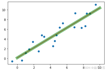
3. 使用TensorFlow实现逻辑回归
实现逻辑回归的套路和实现线性回归差不多, 只不过逻辑回归的目标函数和损失函数不一样而已.
import numpy as np
import matplotlib.pyplot as plt
from sklearn.datasets import make_blobs
import tensorflow as tf


data, target = make_blobs(centers=2)
plt.scatter(data[:, 0], data[:, 1], c=target)

w = tf.Variable(initial_value= np.random.randn(2, 2) * 0.01, dtype=tf.float32)
b = tf.Variable(initial_value=0, dtype=tf.float32)

x = tf.constant(data, dtype=tf.float32)
y = tf.constant(target, dtype=tf.int32)

# 对y做one_hot处理
y  = tf.one_hot(y, depth=2)

# 定义目标函数
def sigmoid(x):
    return tf.nn.sigmoid(tf.matmul(x, w) + b) # (100, 2) * (2, 2) -> (100, 2)

# 定义损失函数
def loss(y_true, y_pred):
    # 对y_pred进行截断
    y_pred = tf.clip_by_value(y_pred, 1e-9, 1)
    return tf.reduce_mean(tf.multiply(y_true, tf.math.log(1/y_pred)))

# 定义优化器
optimizer = tf.optimizers.SGD(0.001)

# 定义优化过程
def run_optimization():
    with tf.GradientTape() as g:
        pred = softmax(x) # shape(100, 1)
        cost = loss(y, pred)

    # 计算梯度
    gradients = g.gradient(cost, [w, b])

    # 更新,w, b
    optimizer.apply_gradients(zip(gradients, [w, b]))


# 计算准确率
def accuracy(y_true, y_pred):
    # 根据阈值对y_pred概率转化成具体类别
    # 100, 2
    # 取最大值的索引
    return tf.reduce_mean(tf.cast(tf.equal(tf.argmax(y_true, 1), tf.argmax(y_pred, axis=1)), dtype=tf.float32))


# 开始训练
for i in range(1, 10000):
    run_optimization()

    if i % 100 == 0:
        y_pred = softmax(x)
        acc = accuracy(y, y_pred)
        loss_ = loss(y, y_pred)
        print(f'准确率: {acc}, 损失: {loss_}')
输出:
准确率: 0.9200000166893005, 损失: 0.3144806921482086
准确率: 0.8999999761581421, 损失: 0.2893371284008026
准确率: 0.9100000262260437, 损失: 0.26885926723480225
准确率: 0.9100000262260437, 损失: 0.25160202383995056
准确率: 0.9200000166893005, 损失: 0.23685793578624725
准确率: 0.9100000262260437, 损失: 0.22414466738700867
准确率: 0.9200000166893005, 损失: 0.21309375762939453
准确率: 0.9200000166893005, 损失: 0.20341530442237854
准确率: 0.9200000166893005, 损失: 0.19487883150577545
准确率: 0.9399999976158142, 损失: 0.1872999519109726
准确率: 0.9399999976158142, 损失: 0.18053019046783447
准确率: 0.9399999976158142, 损失: 0.17444901168346405
...
准确率: 0.949999988079071, 损失: 0.09776999801397324
准确率: 0.949999988079071, 损失: 0.0971640795469284
准确率: 0.949999988079071, 损失: 0.09657695889472961
准确率: 0.949999988079071, 损失: 0.09600784629583359
准确率: 0.949999988079071, 损失: 0.09545581787824631
准确率: 0.949999988079071, 损失: 0.09492019563913345
准确率: 0.949999988079071, 损失: 0.09440017491579056

腾讯云面向开发者汇聚海量精品云计算使用和开发经验,营造开放的云计算技术生态圈。
更多推荐
 30
30 0
0- 0


 已为社区贡献4条内容

所有评论(0)