方法：

当我们使用scene graph generation benchmark 这个项目，进行训练的时候，我们一般会在项目根目录下运行官网上提供的类似于下面这个训练代码：

CUDA_VISIBLE_DEVICES=0,1 python -m torch.distributed.launch --master_port 10025 --nproc_per_node=2 tools/relation_train_net.py --config-file "configs/e2e_relation_X_101_32_8_FPN_1x.yaml" MODEL.ROI_RELATION_HEAD.USE_GT_BOX True MODEL.ROI_RELATION_HEAD.USE_GT_OBJECT_LABEL True MODEL.ROI_RELATION_HEAD.PREDICTOR MotifPredictor SOLVER.IMS_PER_BATCH 12 TEST.IMS_PER_BATCH 2 DTYPE "float16" SOLVER.MAX_ITER 50000 SOLVER.VAL_PERIOD 2000 SOLVER.CHECKPOINT_PERIOD 2000 GLOVE_DIR /home/kaihua/glove MODEL.PRETRAINED_DETECTOR_CKPT /home/kaihua/checkpoints/pretrained_faster_rcnn/model_final.pth OUTPUT_DIR /home/kaihua/checkpoints/motif-precls-exmp

这个代码其中的一些句子命令中（比如下面这三条）我们可以找到一些相关的权重文件夹和输出文件夹：

# glove的权重文件夹
/home/kaihua/glove MODEL.PRETRAINED_DETECTOR_CKPT 
# faster rcnn的权重文件夹
/home/kaihua/checkpoints/pretrained_faster_rcnn/model_final.pth 
# 训练后的输出文件夹
OUTPUT_DIR /home/kaihua/checkpoints/motif-precls-exmp

我们可以从命令OUTPUT_DIR（输出文件夹）的/home/kaihua/checkpoints/motif-precls-exmp这个位置，一步一步继续探索：

比如我现在运行的是causal-motifs模型，我们一步一步可以点进下面的VG_stanford_filtered_with_attribute_test文件夹里

# 文件结构
checkpoints/
causal-motifs-precls-exmp/
inference/
VG_stanford_filtered_with_attribute_test

里面有这三个文件：

eval_results.pytorch  
result_dict.pytorch  
visual_info.json

读取里面的文件内容，这些里面就保存的groundtruth识别的对象结果，预测的faster rcnn识别的对象结果，以及模型训练后生成的三元组。我们只要读取他们就好。

至于读取大家都会吧。两种文件类型。pytorch用这样读取：

 eval_results = torch.load(eval_results_path, map_location=torch.device('cpu'))

json这样读取：

with open(visual_info_path, 'r') as f:
    visual_info_data = json.load(f)

简单提一下使用方法：
比如当我们读取了eval_results.pytorch后: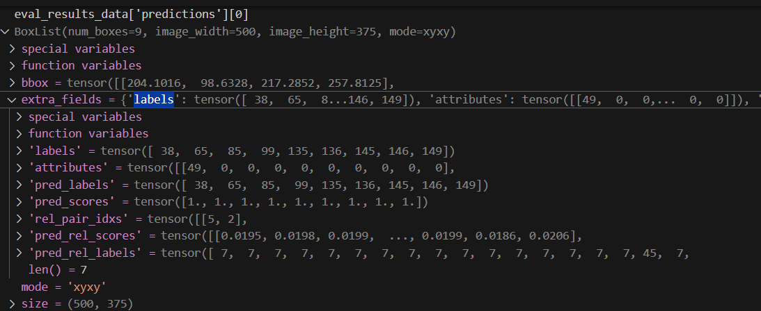

• eval_results_data['predictions'][0]：即预测结果，图片id为0时的数据
• bbox：不用解释了。
• eval_results_data['predictions'][0].extra_fields里：
  • pred_labels和上面的bbox一一对应，是每一个bbox的faster rcnn预测的名词种类id(vg150的150个名词类别排序的id），vg150的150个名词种类我下面贴了，下标从0开始)
  • ['rel_pair_idxs']是上面预测的每一个bounding box的序号的对象对(即主语，宾语组合)，比如[5,2]，就是下标五和下标二这两个bbox的物体组成一个对象对。（序号下标从0开始哦）
  • ['pred_rel_labels'] 和['rel_pair_idxs']一一对应，是这些对象对的预测的关系的种类id，比如7，就是vg150里50个关系词的下标为7的关系词（下标从0开始喔，我下面贴了）。
  • ['pred_rel_scores']是这些预测的关系的置信度打分

大家最好把这些值输出一下，理解一下，比如:
eval_results_data['predictions'][0].extra_fields['rel_pair_idxs'] 的值是：

tensor([[5, 2],
        [1, 2],
        [6, 1],
        [5, 6],
        [5, 3],
        [5, 1],
        [1, 3],
        [1, 6],
        [2, 3],
        [5, 4],
        [1, 7],
        [8, 1],
        [2, 1],
        [6, 5],
        [1, 4],
        [5, 0],
        [4, 2],
        [1, 0],
        [8, 5],
        [6, 2],
        [4, 1],
        [5, 7],
        [1, 5],
        [0, 1],
        [7, 1],
        [8, 2],
        [2, 4],
        [0, 4],
        [2, 6],
        [1, 8],
        [5, 8],
        [0, 5],
        [7, 3],
        [2, 5],
        [6, 4],
        [2, 0],
        [2, 7],
        [4, 5],
        [4, 6],
        [7, 6],
        [8, 7],
        [6, 3],
        [0, 2],
        [8, 6],
        [2, 8],
        [6, 7],
        [4, 3],
        [7, 4],
        [4, 0],
        [3, 1],
        [7, 2],
        [8, 4],
        [6, 0],
        [7, 0],
        [4, 7],
        [0, 7],
        [0, 3],
        [7, 8],
        [0, 6],
        [7, 5],
        [8, 3],
        [3, 2],
        [6, 8],
        [8, 0],
        [3, 7],
        [3, 5],
        [3, 4],
        [4, 8],
        [0, 8],
        [3, 0],
        [3, 6],
        [3, 8]])

比如eval_results_data['predictions'][0].extra_fields['pred_rel_labels']的值是（和上面的对象对一一对应）：

tensor([ 7,  7,  7,  7,  7,  7,  7,  7,  7,  7,  7,  7,  7,  7,  7,  7, 45,  7,
         7,  7, 50,  7,  7,  7, 50,  7,  7,  7,  7,  7,  7,  7,  7,  7,  7,  7,
         7, 50,  7,  7,  7,  7, 45,  7,  7,  7,  7,  7,  7, 45,  7,  7,  7,  7,
        50,  7,  7,  7,  7,  7,  7, 40,  7,  7, 29, 40, 29,  2,  7, 29, 29, 40])

关系三元组是怎么从序号换算的？

1. 比如image_id = 1的图片，其prediction_obj.extra_fields['labels']的值是： ([ 4,23, 23, 31, 87, 99, 105, 114, 115, 145, 149]) 。这是每个bounding box对应的物体的类别（参考vg150的150个物体）。
2. 现在prediction_obj.extra_fields['rel_pair_idxs']里的第一个物体对是 [5,2]。
3. 再参考prediction_obj.extra_fields['labels']的值，发现这个物体对是[99,23](下标从0开始），之后去vg150的150个名词里去找，发现[99,23]对应的物体对是[pole,bus]（下面我贴了vg150的150个名词类别）。
4. 再结合prediction_obj.extra_fields['pred_rel_labels']中的值，发现关系是7，这个三元组是[5,7,2],7在vg150的50个关系中是attached to（关系词下标从1开始而不是从0开始），所以这个预测的三元组是[pole,attached to,bus]。

最后贴一下vg150的150个名词和50个关系词
(注意，这里我已经去掉了background背景，换算读取时从下标0开始)

# 定义 150 个名词类别
NOUN_CATEGORIES = [
    'airplane', 'animal', 'arm', 'bag', 'banana', 'basket', 'beach', 'bear', 'bed', 'bench', 'bike', 'bird', 'board', 'boat', 'book', 'boot', 'bottle', 'bowl', 'box', 'boy', 'branch', 'building', 'bus', 'cabinet', 'cap', 'car', 'cat', 'chair', 'child', 'clock', 'coat', 'counter', 'cow', 'cup', 'curtain', 'desk', 'dog', 'door', 'drawer', 'ear', 'elephant', 'engine', 'eye', 'face', 'fence', 'finger', 'flag', 'flower', 'food', 'fork', 'fruit', 'giraffe', 'girl', 'glass', 'glove', 'guy', 'hair', 'hand', 'handle', 'hat', 'head', 'helmet', 'hill', 'horse', 'house', 'jacket', 'jean', 'kid', 'kite', 'lady', 'lamp', 'laptop', 'leaf', 'leg', 'letter', 'light', 'logo', 'man', 'men', 'motorcycle', 'mountain', 'mouth', 'neck', 'nose', 'number', 'orange', 'pant', 'paper', 'paw', 'people', 'person', 'phone', 'pillow', 'pizza', 'plane', 'plant', 'plate', 'player', 'pole', 'post', 'pot', 'racket', 'railing', 'rock', 'roof', 'room', 'screen', 'seat', 'sheep', 'shelf', 'shirt', 'shoe', 'short', 'sidewalk', 'sign', 'sink', 'skateboard', 'ski', 'skier', 'sneaker', 'snow', 'sock', 'stand', 'street', 'surfboard', 'table', 'tail', 'tie', 'tile', 'tire', 'toilet', 'towel', 'tower', 'track', 'train', 'tree', 'truck', 'trunk', 'umbrella', 'vase', 'vegetable', 'vehicle', 'wave', 'wheel', 'window', 'windshield', 'wing', 'wire', 'woman', 'zebra'
]

# 预定义的50种关系词类别如下：
RELATIONSHIP_CATEGORIES = [
    'above', 'across', 'against', 'along', 'and', 'at', 'attached to', 'behind',
    'belonging to', 'between', 'carrying', 'covered in', 'covering', 'eating',
    'flying in', 'for', 'from', 'growing on', 'hanging from', 'has', 'holding',
    'in', 'in front of', 'laying on', 'looking at', 'lying on', 'made of',
    'mounted on', 'near', 'of', 'on', 'on back of', 'over', 'painted on',
    'parked on', 'part of', 'playing', 'riding', 'says', 'sitting on',
    'standing on', 'to', 'under', 'using', 'walking in', 'walking on',
    'watching', 'wearing', 'wears', 'with'
]

其实visio_info.json这个文件也挺重要的。

比如我们读取后：
visual_info_data[1][‘prediction’]的值是：

[
[96.6796875, 278.80859375, 121.09375, 306.15234375, 'bag'],
[332.51953125, 123.53515625, 498.53515625, 229.00390625, 'bus'],
[32.2265625, 88.8671875, 495.60546875, 287.109375, 'bus'],
[103.02734375, 183.10546875, 198.2421875, 275.390625, 'coat'],
[123.046875, 264.16015625, 179.19921875, 355.46875, 'pant'],
[87.40234375, 50.29296875, 94.7265625, 310.546875, 'pole'],
[2.9296875, 0.9765625, 497.0703125, 125.0, 'roof'], 
[0.9765625, 207.51953125, 235.3515625, 373.53515625, 'sidewalk'],
[40.0390625, 41.50390625, 93.26171875, 101.5625, 'sign'],
[38.0859375, 129.8828125, 123.53515625, 193.359375, 'window'],
[97.16796875, 161.62109375, 193.359375, 358.88671875, 'woman']]

很清晰很明显，哪个bbox对应哪个物体，直接就给出来了。就不用按上面eval_results.pytorch里，先把对象对，换算成哪一个bounding box，再把这个bounding box，换算成名词的种类，再去对应三元组了。很省事

后续：

1. 我本来想这样保存结果：
   • 测试代码运行了tools/relation_test_net.py脚本。这个脚本里，模型会对训练好的图像的三元组进行深度学习的打分处理。
   • 我本来想着，在脚本的主测试循环中，初始化一个空的 Python 列表，用于存储所有图像的预测三元组结果。之后在测试循环的每次迭代中，模型会对一批(一个batch)图像进行打分。每次我们获取一个batch的模型输出。

但感觉也太麻烦了。后来发现原来直接读取训练后的输出文件夹里的文件内容就可以了。