一、Tensor概述

PyTorch会将数据封装成张量（Tensor）进行计算，所谓张量就是元素为相同类型的多维矩阵。

张量可以在 GPU 上加速运行。

1、概念

张量是一个多维数组，通俗来说可以看作是扩展了标量、向量、矩阵的更高维度的数组。张量的维度决定了它的形状（Shape），例如：

• 标量 是 0 维张量，如 a = torch.tensor(5)

• 向量 是 1 维张量，如 b = torch.tensor([1, 2, 3])

• 矩阵 是 2 维张量，如 c = torch.tensor([[1, 2], [3, 4]])

• 更高维度的张量，如3维、4维等，通常用于表示图像、视频数据等复杂结构。

2、特点

• 动态计算图：PyTorch 支持动态计算图，这意味着在每一次前向传播时，计算图是即时创建的。

• GPU 支持：PyTorch 张量可以通过 .to('cuda') 移动到 GPU 上进行加速计算。

• 自动微分：通过 autograd 模块，PyTorch 可以自动计算张量运算的梯度，这对深度学习中的反向传播算法非常重要。

3、数据类型

PyTorch中有3种数据类型：浮点数、整数、布尔。其中，浮点数和整数又分为8位、16位、32位、64位，加起来共9种。

为什么要分为8位、16位、32位、64位呢？

场景不同，对数据的精度和速度要求不同。通常，移动或嵌入式设备追求速度，对精度要求相对低一些。精度越高，往往效果也越好，自然硬件开销就比较高。

二、Tensor的创建

在Torch中张量以 "类" 的形式封装起来，对张量的一些运算、处理的方法被封装在类中，官方文档：

torch — PyTorch 2.7 documentation

1、基础创建方式

以下讲的创建tensor的函数中有两个有默认值的参数dtype和device, 分别代表数据类型和计算设备，可以通过属性dtype和device获取。

1.1 torch.tensor

torch.tensor(数据，dtpye=  ，device='  ')

注意这里的tensor是小写，该API是根据指定的数据创建张量。

import torch

# 使用tensor()创建张量，可创建标量、一维、二维、多维数组
# 参数：
# dtype：指定张量的数据类型
# device：指定张量的运算设备，默认为CPU
def test01():
    t1=torch.tensor([1,2,3],dtype=torch.float32,device='cuda')
    print(t1)
    # size()和shape作用一样，获取张量形状
    print(t1.size())
    # dtype：获取张量的数据类型，如果再创建张量时没有指定dtype，则自动根据输入数组的数据类型判断
    print(t1.dtype)

if __name__ == '__main__':
    test01()

 输出

tensor([1., 2., 3.], device='cuda:0')
torch.Size([3])
torch.float32

1.2 torch.Tensor

torch.Tensor()

注意这里的Tensor是大写，该API根据形状创建张量，其也可用来创建指定数据的张量。

import torch

# 使用Tensor()构造函数创建张量
# 强制将数据类型转换为float32
# 没有dtype和device属性
# tensor()创建张量更灵活，使用更多一些
def test02():
    t1=torch.Tensor([1,2,3])
    print(t1)
    print(t1.dtype)
    print(t1.size())

if __name__ == '__main__':
    test02()

输出 

tensor([1., 2., 3.])
torch.float32
torch.Size([3])

1.3 torch.IntTensor

用于创建指定类型的张量，还有诸如Torch.FloatTensor、 torch.DoubleTensor、 torch.LongTensor......等。

如果数据类型不匹配，那么在创建的过程中会进行类型转换，要尽可能避免，防止数据丢失。

2、创建线性和随机张量

在 PyTorch 中，可以轻松创建线性张量和随机张量。

2.1创建线性张量

torch.arange(起始值，终止值，步长) 不含终止值

torch.linspace(起始值，终止值，步长) 含终止值

import torch
import numpy as np

# 不用科学计数法打印
torch.set_printoptions(sci_mode=False)


def test004():
    # 1. 创建线性张量
    r1 = torch.arange(0, 10, 2)
    print(r1)
    # 2. 在指定空间按照元素个数生成张量：等差
    r2 = torch.linspace(3, 10, 10)
    print(r2)
    
    r2 = torch.linspace(3, 10000000, 10)
    print(r2)
    

if __name__ == "__main__":
    test004()

输出 

tensor([0, 2, 4, 6, 8])
tensor([ 3.0000,  3.7778,  4.5556,  5.3333,  6.1111,  6.8889,  7.6667,  8.4444,
         9.2222, 10.0000])
tensor([    3.0000, 1111113.7500, 2222224.5000, 3333335.2500, 4444446.0000, 5555557.0000,
        6666668.0000, 7777778.5000, 8888889.0000, 10000000.0000])

2.2随机张量

torch.rand() 随机张量

torch.randn() 符合标准正态分布的随机数

torch.manul_seed(）设置随机数种子

import torch

def test01():
    # 设置随机数种子，目的使每次运行程序产生的随机数都相同，随机数种子是int类型，可以随便设置，如0,42,123等都可以
    torch.manual_seed(0)
    s=torch.randint(0,10,(2,3))
    print(s)

    # randn：符合标准正态分布的随机数，均值为0，标准差为1
    s1=torch.randn(2,3)
    print(s1)

if __name__ == '__main__':
    test01()

输出

tensor([[4, 9, 3],
        [0, 3, 9]])
tensor([[ 1.2645, -0.6874,  0.1604],
        [-0.6065, -0.7831,  1.0622]])

三、Tensor常见属性

1、获取属性

变量.dtype 数据类型

变量.device 运行设备

变量.shape 形状

import torch


def test001():
    data = torch.tensor([1, 2, 3])
    print(data.dtype, data.device, data.shape)


if __name__ == "__main__":
    test001()

输出

torch.int64 cpu torch.Size([3])

2、切换设备

torch.tensor(device='  ')

变量.to('  ')

变量.cpu()   变量.cuda()

import torch

def test01():
    # 在创建张量时指定device
    t1=torch.tensor([1,2,3],device='cuda')
    print(t1)

    # 使用to()方法切换设备,转换后要重新赋值变量
    t2=torch.tensor([1,2,3])
    t2=t2.to('cuda')
    print(t2.device)

    # 使用cuda()或cpu()切换运算设备
    t3=torch.tensor([1,2,3],device='cuda')
    t3=t3.cpu()
    print(t3.device)
    t3=t3.cuda()
    print(t3.device)


if __name__ == '__main__':
    test01()

3、类型转换

在训练模型或推理时，类型转换也是张量的基本操作，是需要掌握的。

import torch


def test001():
    data = torch.tensor([1, 2, 3])
    print(data.dtype)  # torch.int64

    # 1. 使用type进行类型转换
    data = data.type(torch.float32)
    print(data.dtype)  # float32
    data = data.type(torch.float16)
    print(data.dtype)  # float16

    # 2. 使用类型方法
    data = data.float()
    print(data.dtype)  # float32
    # 16 位浮点数，torch.float16，即半精度
    data = data.half()
    print(data.dtype)  # float16
    data = data.double()
    print(data.dtype)  # float64
    data = data.long()
    print(data.dtype)  # int64
    data = data.int()
    print(data.dtype)  # int32

    #  使用dtype属性
    data = torch.tensor([1, 2, 3], dtype=torch.half)
    print(data.dtype)


if __name__ == "__main__":
    test001()

四、Tensor数据转换

1、tensor转numpy

浅拷贝：变量.numpy()

深拷贝：变量.numpy().copy()

import torch
import numpy as np

# tensor转numpy:numpy()
def test01():
    t1=torch.tensor([[1,2,3],[4,5,6]])
    print(t1)
    # 浅拷贝
    n1=t1.numpy()
    print(n1)

    # 深拷贝
    n2=t1.numpy().copy()
    print(n2)

if __name__=='__main__':
    test01()

 输出

tensor([[1, 2, 3],
        [4, 5, 6]])
[[1 2 3]
 [4 5 6]]
[[1 2 3]
 [4 5 6]]

2、 numpy转tensor

浅拷贝：torch.from_numpy()

深拷贝：torch.tensor()

import torch
import numpy as np

# numpy转化为tensor
# 浅拷贝：torch.from_numpy() 数组内存共享
# 深拷贝：torch.tensor() 参数为numpy数组，创建新的副本
def test02():
    n1=np.array([1,2,3,4,5])
    t1=torch.from_numpy(n1)
    print(t1)

    t2=torch.tensor(n1)
    print(t2)

if __name__=='__main__':
    test02()

输出

tensor([1, 2, 3, 4, 5], dtype=torch.int32)
tensor([1, 2, 3, 4, 5], dtype=torch.int32)

五、Tensor常见操作

在深度学习中，Tensor是一种多维数组，用于存储和操作数据，我们需要掌握张量各种运算。

1、获取元素值

我们可以把单个元素tensor转换为Python数值，这是非常常用的操作

变量.item()

import torch

# item():从单个元素的tensor中获取标量值
# 获取元素和tensor的维度没有关系，只要tensor只有一个元素，都可以使用该方法获取值
def test01():
    t1=torch.tensor(18)
    print(t1.item())

    t2=torch.tensor([[19]])
    print(t2.item())

if __name__ == '__main__':
    test01()

输出

18
19

2、元素值运算

常见的加减乘除次方取反开方等各种操作，带有_的方法则会替换原始值。

import torch


def test001():
    # 生成范围 [0, 10) 的 2x3 随机整数张量
    data = torch.randint(0, 10, (2, 3))
    print(data)
    # 元素级别的加减乘除：不修改原始值
    print(data.add(1))
    print(data.sub(1))
    print(data.mul(2))
    print(data.div(3))
    print(data.pow(2))

    # 元素级别的加减乘除：修改原始值
    data = data.float()
    data.add_(1)
    data.sub_(1)
    data.mul_(2)
    data.div_(3.0)
    data.pow_(2)
    print(data)


if __name__ == "__main__":
    test001()

3、阿达玛积和Tensor矩阵相乘

import torch


# 阿达玛积：两个相同形状的矩阵相同位置的元素相乘，得出的新矩阵
# 矩阵相乘：(m,p)和(p,n)形状的矩阵相乘，结果为(m,n)，运算符合：matmull或@
def test02():
    t1=torch.tensor([[2,3],[4,5]])
    t2=torch.tensor([[1,2],[3,4]])
    # 阿达玛积
    print(t1*t2)
    # 矩阵相乘
    print(t1@t2)

if __name__ == '__main__':
    test02()

输出

tensor([[ 2,  6],
        [12, 20]])
tensor([[11, 16],
        [19, 28]])

4、形状操作

4.1view()和reshape()

在 PyTorch 中，张量的形状操作是非常重要的，因为它允许你灵活地调整张量的维度和结构，以适应不同的计算需求。

将张量转换为不同的形状，但要确保转换后的形状与原始形状具有相同的元素数量。

view() 数据必须是连续的

reshape()

import torch

# view：张量变形，和reshape()类似
# 和reshape区别：
# view():前提是数据在内存中是连续的，即按c顺序存储
# view效率比reshape高
# 如果数据不连续，使用view()会报错，可以使用reshape代替
def test03():
    t1=torch.tensor([[1,2,3],[4,5,6]])
    print(t1.is_contiguous())
    t2=t1.view(3,-1)
    print(t2.is_contiguous())

    t3=t1.t()
    print(t3.is_contiguous())
    t4=t3.view(2,-1)
    print(t4)

if __name__ == '__main__':
    test03()

4.2升维和降维

降维：torch.squeeze(dim=  ) 降维度为1的

升维：torch.unsqueeze(dim=  )

# 升维和降维
# 升维：unsqueeze()
# 降维：squeeze()
# 使用场景：一般在图形图像处理上，添加或删除维度
def test05():
    t1=torch.randint(1,10,(2,3,4))
    # 升维
    t2=torch.unsqueeze(t1,dim=0)
    print(t2.size())
    # 升维方式2
    t2=t1.unsqueeze(0)
    print(t2.size())

    # 降维
    # 1.如果不指定dim，默认删除所有维度为1的维度
    # 2.如果指定dim的维度不为1，则不做任何操作，也不报错
    t3=torch.squeeze(t2,dim=1)
    print(t3.size())

if __name__ == '__main__':
    test05()

输出

torch.Size([1, 2, 3, 4])
torch.Size([1, 2, 3, 4])
torch.Size([1, 2, 3, 4])

5、广播机制

广播机制允许在对不同形状的张量进行计算，而无需显式地调整它们的形状。广播机制通过自动扩展较小维度的张量，使其与较大维度的张量兼容，从而实现按元素计算。

规则

广播机制需要遵循以下规则：

• 每个张量的维度至少为1

• 满足右对齐

六、自动微分

自动微分模块torch.autograd负责自动计算张量操作的梯度，具有自动求导功能。自动微分模块是构成神经网络训练的必要模块，可以实现网络权重参数的更新，使得反向传播算法的实现变得简单而高效。

1、基础概念

• 张量

Torch中一切皆为张量，属性requires_grad决定是否对其进行梯度计算。默认是 False，如需计算梯度则设置为True。

• 计算图

torch.autograd通过创建一个动态计算图来跟踪张量的操作，每个张量是计算图中的一个节点，节点之间的操作构成图的边。

在 PyTorch 中，当张量的 requires_grad=True 时，PyTorch 会自动跟踪与该张量相关的所有操作，并构建计算图。每个操作都会生成一个新的张量，并记录其依赖关系。当设置为 True 时，表示该张量在计算图中需要参与梯度计算，即在反向传播（Backpropagation）过程中会自动计算其梯度；当设置为 False 时，不会计算梯度。

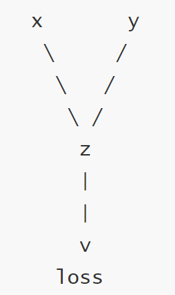
例如：z=x*y      loss=z.sum()

在上述代码中，x 和 y 是输入张量，即叶子节点，z 是中间结果，loss 是最终输出。每一步操作都会记录依赖关系：

z = x * y：z 依赖于 x 和 y。

loss = z.sum()：loss 依赖于 z。

这些依赖关系形成了一个动态计算图，如下所示：

• 叶子节点

在 PyTorch 的自动微分机制中，叶子节点（leaf node） 是计算图中：

• 由用户直接创建的张量，并且它的 requires_grad=True。

• 这些张量是计算图的起始点，通常作为模型参数或输入变量。

特征：

• 没有由其他张量通过操作生成。

• 如果参与了计算，其梯度会存储在 leaf_tensor.grad 中。

• 默认情况下，叶子节点的梯度不会自动清零，需要显式调用 optimizer.zero_grad() 或 x.grad.zero_() 清除。

• 反向传播

使用tensor.backward()方法执行反向传播，从而计算张量的梯度。这个过程会自动计算每个张量对损失函数的梯度。例如：调用 loss.backward() 从输出节点 loss 开始，沿着计算图反向传播，计算每个节点的梯度。

• 梯度

计算得到的梯度通过tensor.grad访问，这些梯度用于优化模型参数，以最小化损失函数。

2、计算梯度

使用tensor.backward()方法执行反向传播，从而计算张量的梯度

2.1标量梯度计算

import torch

# 自动求导：
# 1.叶子节点张量要添加requires_grad= True
# 2.叶子节点的数据类型是浮点数
# 3.调用backward()可以自动求导
# 4.求导后的梯度保存在叶子节点的grad属性中
def test01():
    x=torch.tensor(1,dtype=torch.float32,requires_grad= True)
    y=x**2
    # 反向传播，做自动求导
    y.backward()
    print(x.grad)

if __name__ == '__main__':
    test01()

tensor(2.) 

2.2向量梯度计算

import torch

def test02():
    x=torch.tensor([1,2,3],requires_grad= True,dtype=torch.float32)
    y=x**2
    # 1.梯度向量，用来对一维向量进行反向传播
    # y.backward(torch.tensor([1.0,1.0,1.0]))
    # 2.把梯度向量通过类似计算损失的方式将输出转化为标量，然后再调用backward()，常用的方式
    z=y.sum()
    z.backward()
    print(x.grad)

if __name__ == '__main__':
    test03()

tensor([2., 4., 6.])

2.3多标量梯度计算

import torch


def test003():
    # 1. 创建两个标量
    x1 = torch.tensor(5.0, requires_grad=True, dtype=torch.float64)
    x2 = torch.tensor(3.0, requires_grad=True, dtype=torch.float64)

    # 2. 构建运算公式
    y = x1**2 + 2 * x2 + 7
    
    # 3. 计算梯度，也就是反向传播
    y.backward()
    
    # 4. 读取梯度值
    print(x1.grad, x2.grad)
    
    # 输出：
    # tensor(10., dtype=torch.float64) tensor(2., dtype=torch.float64)


if __name__ == "__main__":
    test003()

2.4多向量梯度计算

import torch

def test03():
    x=torch.tensor([1,2,3],requires_grad= True,dtype=torch.float32)
    y=torch.tensor([2,3,4],requires_grad= True,dtype=torch.float32)
    z=x*y
    loss=z.sum()
    loss.backward()
    print(x.grad,y.grad)
    print(z.grad)

if __name__ == '__main__':
    test03()

 tensor([2., 3., 4.]) tensor([1., 2., 3.])
None

3、梯度上下文控制

梯度计算的上下文控制和设置对于管理计算图、内存消耗、以及计算效率至关重要。下面我们学习下Torch中与梯度计算相关的一些主要设置方式。

3.1控制梯度计算

with torch.no_grad():

        表达式

import torch

def test04():
    x=torch.tensor([1,2,3],requires_grad= True,dtype=torch.float32)
    # torch.no_grad():禁止该上下文的代码参与梯度计算
    with torch.no_grad():
        y=x**2

if __name__ == '__main__':
    test04()

 False

import torch


def test001():
    x = torch.tensor(10.5, requires_grad=True)
    print(x.requires_grad)  # True

    # 1. 默认y的requires_grad=True
    y = x**2 + 2 * x + 3
    print(y.requires_grad)  # True

    # 2. 如果不需要y计算梯度-with进行上下文管理
    with torch.no_grad():
        y = x**2 + 2 * x + 3
    print(y.requires_grad)  # False

    # 3. 如果不需要y计算梯度-使用装饰器
    @torch.no_grad()
    def y_fn(x):
        return x**2 + 2 * x + 3

    y = y_fn(x)
    print(y.requires_grad)  # False

    # 4. 如果不需要y计算梯度-全局设置，需要谨慎
    torch.set_grad_enabled(False)
    y = x**2 + 2 * x + 3
    print(y.requires_grad)  # False


if __name__ == "__main__":
    test001()

3.2累计梯度

pytorch中累计梯度为累加

import torch

def test05():
    x=torch.tensor([1,2,3],requires_grad= True,dtype=torch.float32)

    # x和y映射函数要放在循环内部
    # 计算途中叶子节点的梯度默认是累加的
    # 不希望叶子节点的梯度累加，需要对每轮次的梯度进行清零
    for epoch in range(5):
        y = x ** 2
        z = y.sum()
        z.backward()
        print(x.grad)

if __name__ == '__main__':
    test05()

tensor([2., 4., 6.])
tensor([ 4.,  8., 12.])
tensor([ 6., 12., 18.])
tensor([ 8., 16., 24.])
tensor([10., 20., 30.])

3.3梯度清零

if 参数.grad is not None:

        参数.grad.zero_()

import torch

def test05():
    x=torch.tensor([1,2,3],requires_grad= True,dtype=torch.float32)

    # x和y映射函数要放在循环内部
    # 计算途中叶子节点的梯度默认是累加的
    # 不希望叶子节点的梯度累加，需要对每轮次的梯度进行清零
    for epoch in range(5):
        y = x ** 2
        z = y.sum()
        # 梯度清零，一般在backward()前执行
        if x.grad is not None:
            x.grad.zero_()
        z.backward()
        print(x.grad)

if __name__ == '__main__':
    test05()

tensor([2., 4., 6.])
tensor([2., 4., 6.])
tensor([2., 4., 6.])
tensor([2., 4., 6.])
tensor([2., 4., 6.])

3.4求函数最小值

import torch
from matplotlib import pyplot as plt

# 求函数最小值
def test06():
    x_list=[]
    y_list=[]
    x=torch.tensor(3.0,requires_grad=True)

    epochs=500
    lr=0.1
    for epoch in range(epochs):
        y=x**2
        z=y.sum()
        # 梯度清零
        if x.grad is not None:
            x.grad.zero_()
        z.backward()
        # 在通过梯度下降公式进行更新时，不参与梯度计算
        # 计算途中的叶子节点不允许直接修改值，需要通过 torch.no_grad()上下文控制器进行更新x值
        with torch.no_grad():
            x-=lr*x.grad

        x_list.append(x.item())
        y_list.append(y.item())

    plt.scatter(x_list,y_list)
    plt.show()

if __name__ == '__main__':
    test06()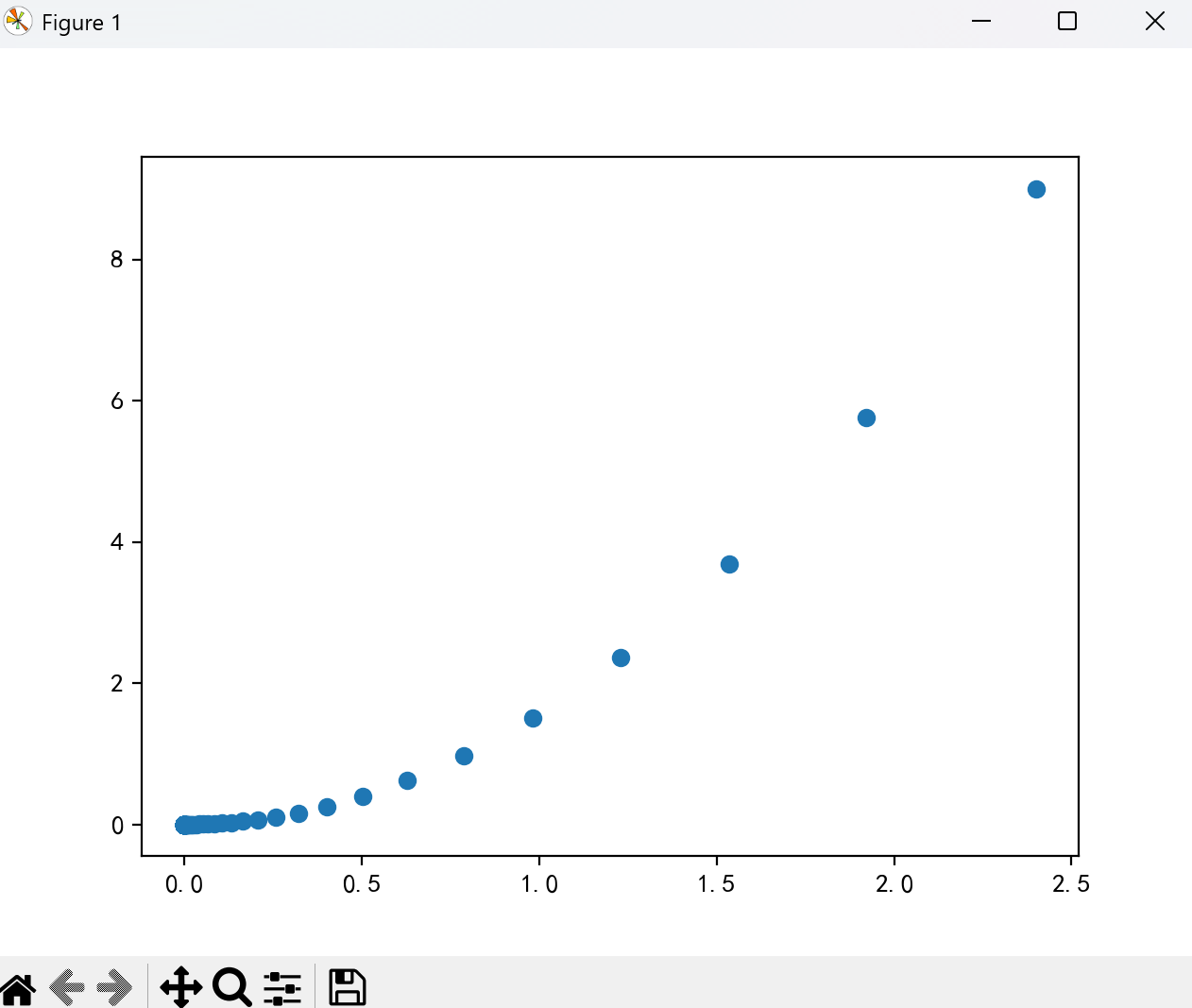

 

3.5函数参数求解

import torch

def test():
    x=torch.tensor([1,2,3,4,5],dtype=torch.float32)
    y=torch.tensor([3,5,7,9,11],dtype=torch.float32)

    a=torch.tensor(1.0,requires_grad=True)
    b=torch.tensor(1.0,requires_grad=True)
    lr=0.01
    epochs=1000
    for epoch in range(epochs):
        y_pred=a*x+b
        loss=torch.mean((y-y_pred)**2)
        if a.grad is not None and b.grad is not None:
            a.grad.data.zero_()
            b.grad.data.zero_()
        loss.backward()

        with torch.no_grad():
            a-=lr*a.grad
            b-=lr*b.grad
        if epoch%100==0:
            print(f'epoch:{epoch+1},a:{a.item()},b:{b.item()}')
    print(f'a:{a.item()},b:{b.item()}')

if __name__ == '__main__':
    test()

epoch:1,a:1.2200000286102295,b:1.059999942779541
epoch:101,a:1.9493879079818726,b:1.1827253103256226
epoch:201,a:1.963927984237671,b:1.1302316188812256
epoch:301,a:1.9742909669876099,b:1.092818021774292
epoch:401,a:1.9816765785217285,b:1.0661531686782837
epoch:501,a:1.9869405031204224,b:1.0471489429473877
epoch:601,a:1.990692377090454,b:1.0336037874221802
epoch:701,a:1.9933662414550781,b:1.0239497423171997
epoch:801,a:1.9952718019485474,b:1.0170700550079346
epoch:901,a:1.996630072593689,b:1.0121663808822632
a:1.9975899457931519,b:1.0087010860443115