1.项目结构如下

data文件夹存放清华的数据集，清华数据集原本有35个被试，这里选择了6个被试。

2.Dataset.py ：数据加载与处理

import scipy.io
import numpy as np
import torch
from scipy import signal


class getSSVEPWithin:
    def __init__(self, subject=1):
        super(getSSVEPWithin, self).__init__()
        self.Nh = 240  # number of trials
        self.Nc = 9  # number of channels
        self.Nt = 500  # number of time points 采样点
        self.Nf = 40  # number of target frequency
        self.Fs = 250  # Sample Frequency
        self.subject = subject  # current subject
        self.data_folds = None

        # 在初始化时加载数据
        self.load_data()

    def load_data(self):
        """加载并处理数据，生成data_folds"""
        subjectfile = scipy.io.loadmat(f'./data/S{self.subject}.mat')
        data_array = subjectfile['data']

        ##########################################################################
        # 对数据做8-64Hz滤波处理
        # 数据维度说明: (64通道, 1500时间点, 40试验, 6块)
        n_channels, n_timepoints, n_trials, n_blocks = data_array.shape

        # 参数设置
        sfreq = 250  # 采样频率 (Hz)，根据5秒时长和1500个点计算

        # 设计带通滤波器 (8-64 Hz)
        nyquist = sfreq / 2
        lowcut = 8 / nyquist
        highcut = 64 / nyquist

        # 4阶巴特沃斯滤波器
        b, a = signal.butter(4, [lowcut, highcut], btype='band')

        # 滤波处理
        data_filtered = np.zeros_like(data_array)
        for block in range(n_blocks):
            for trial in range(n_trials):
                for channel in range(n_channels):
                    data_filtered[channel, :, trial, block] = signal.filtfilt(
                        b, a, data_array[channel, :, trial, block]
                    )  # (64, 1500, 40, 6)

        ##########################################################################
        # 数据格式转换
        data_filtered = data_filtered.reshape(64, 1500, -1)  # (64, 1500, 40, 6)->(64, 1500, 240)

        # 选取枕区9个通道
        part1 = data_filtered[47:48, :, :]
        part2 = data_filtered[53:58, :, :]
        part3 = data_filtered[60:63, :, :]

        # 把选取的9个通道合并
        samples = np.concatenate([part1, part2, part3], axis=0)

        # 采样点取段
        samples = samples[:, 160:660, :]  # 取500个采样点
        eeg_data = samples.swapaxes(1, 2)  # (9, 500, 240) -> (9, 240, 500)
        eeg_data = torch.from_numpy(eeg_data.swapaxes(0, 1))  # (9, 240, 500) -> (240, 9, 500)
        eeg_data = eeg_data.reshape(-1, 1, self.Nc, self.Nt)  # (240, 1, 9, 500)

        ##########################################################################
        # 生成数据标签
        labels = []
        # 对于每个类别（40个），每个类别有6个试次
        for class_label in range(40):  # 40个类别
            for trial in range(6):  # 每个类别6个试次
                labels.append(class_label + 1)  # 标签从1开始（1-40）

        labels_array = np.array(labels).reshape(-1, 1)  # (240, 1)
        label_data = torch.from_numpy(labels_array)
        label_data = label_data-1#让数据标签从0开始


        ##########################################################################
        # 划分数据集为6折
        data_folds = []

        for test_trial in range(6):  # 6个试次，每个作为一次测试集
            # 测试集索引：每个类别的第test_trial个试次
            test_indices = []
            train_indices = []

            for class_idx in range(40):  # 40个类别
                base_idx = class_idx * 6  # 每个类别的起始索引

                # 测试集：该类别的第test_trial个试次
                test_idx = base_idx + test_trial
                test_indices.append(test_idx)

                # 训练集：该类别的其他5个试次
                for trial in range(6):
                    if trial != test_trial:
                        train_idx = base_idx + trial
                        train_indices.append(train_idx)

            # 获取训练集和测试集数据
            train_data_fold = eeg_data[train_indices]
            train_labels_fold = label_data[train_indices]
            test_data_fold = eeg_data[test_indices]
            test_labels_fold = label_data[test_indices]

            # 确保数据格式不变
            train_data_fold = train_data_fold.reshape(-1, 1, 9, 500)
            test_data_fold = test_data_fold.reshape(-1, 1, 9, 500)
            train_labels_fold = train_labels_fold.reshape(-1, 1)
            test_labels_fold = test_labels_fold.reshape(-1, 1)

            # 存储该折的数据
            fold_data = {
                'train_data': train_data_fold,  # torch.Tensor, shape: (200, 1, 9, 500)
                'train_labels': train_labels_fold,  # torch.Tensor, shape: (200, 1)
                'test_data': test_data_fold,  # torch.Tensor, shape: (40, 1, 9, 500)
                'test_labels': test_labels_fold,  # torch.Tensor, shape: (40, 1)
                'fold_idx': test_trial
            }

            data_folds.append(fold_data)

        self.data_folds = data_folds

    def getData(self):
        """返回处理好的data_folds"""
        if self.data_folds is None:
            self.load_data()
        return self.data_folds

    def get_fold(self, fold_idx):
        """获取指定折的数据"""
        if self.data_folds is None:
            self.load_data()
        if 0 <= fold_idx < len(self.data_folds):
            return self.data_folds[fold_idx]
        else:
            raise ValueError(f"fold_idx must be between 0 and {len(self.data_folds) - 1}")

    def __len__(self):
        """返回折数"""
        if self.data_folds is None:
            self.load_data()
        return len(self.data_folds)

    def __getitem__(self, idx):
        """通过索引访问折数据"""
        if self.data_folds is None:
            self.load_data()
        return self.data_folds[idx]

3.CNN.py ：卷积神经网络模块

import torch.nn as nn

# 定义卷积神经网络模型
class CNN(nn.Module):
    """
    EEG分类CNN网络
    输入形状: (batch_size, 1, 9, 500)
    输出: 40个类别的概率
    """

    def __init__(self, num_classes=40):
        super(CNN, self).__init__()

        # 第一个卷积块
        self.conv1 = nn.Sequential(
            nn.Conv2d(1, 32, kernel_size=(1, 5), padding=(0, 2)),
            nn.BatchNorm2d(32),
            nn.ELU(inplace=True),
            nn.Dropout(0.3)
        )

        # 第二个卷积块 - 空间卷积
        self.conv2 = nn.Sequential(
            nn.Conv2d(32, 32, kernel_size=(9, 1), padding=(0, 0)),
            nn.BatchNorm2d(32),
            nn.ELU(inplace=True),
            nn.Dropout(0.3),
            nn.AvgPool2d(kernel_size=(1, 4))
        )

        # 第三个卷积块
        self.conv3 = nn.Sequential(
            nn.Conv2d(32, 64, kernel_size=(1, 5), padding=(0, 2)),
            nn.BatchNorm2d(64),
            nn.ELU(inplace=True),
            nn.Dropout(0.3),
            nn.AvgPool2d(kernel_size=(1, 4))
        )

        # 第四个卷积块
        self.conv4 = nn.Sequential(
            nn.Conv2d(64, 128, kernel_size=(1, 5), padding=(0, 2)),
            nn.BatchNorm2d(128),
            nn.ELU(inplace=True),
            nn.Dropout(0.3),
            nn.AvgPool2d(kernel_size=(1, 2))
        )

        # 计算全连接层输入尺寸
        # 经过conv2后: (1, 500) -> (1, 125) [500/4]
        # 经过conv3后: (1, 125) -> (1, 31) [125/4]
        # 经过conv4后: (1, 31) -> (1, 15) [31/2]
        # 最终: 128 * 1 * 15 = 1920

        # 全连接层
        self.fc = nn.Sequential(
            nn.Linear(128 * 1 * 15, 512),
            nn.ELU(inplace=True),
            nn.Dropout(0.5),
            nn.Linear(512, num_classes)
        )

    def forward(self, x):
        # x形状: (batch, 1, 9, 500)
        x = self.conv1(x)  # -> (batch, 32, 9, 500)
        x = self.conv2(x)  # -> (batch, 32, 1, 125)
        x = self.conv3(x)  # -> (batch, 64, 1, 31)
        x = self.conv4(x)  # -> (batch, 128, 1, 15)

        # 展平
        x = x.view(x.size(0), -1)  # -> (batch, 128*1*15)
        x = self.fc(x)  # -> (batch, 40)

        return x

3.Train_Within.py ：模型训练，6折交叉验证

import torch
import torch.nn as nn
import torch.optim as optim
from torch.utils.data import DataLoader, TensorDataset
import numpy as np
import matplotlib.pyplot as plt
import Dataset as Dataset
import CNN
import warnings
from sklearn.metrics import accuracy_score, confusion_matrix

# 忽略所有警告
warnings.filterwarnings('ignore')
# 训练函数
def train_one_epoch(model, train_loader, criterion, optimizer, device):
    """训练一个epoch"""
    model.train()
    total_loss = 0
    all_preds = []
    all_labels = []

    for batch_idx, (data, labels) in enumerate(train_loader):
        data = data.to(device).float()
        labels = labels.to(device).squeeze().long()  # 去掉多余的维度

        # 前向传播
        outputs = model(data)
        loss = criterion(outputs, labels)

        # 反向传播
        optimizer.zero_grad()
        loss.backward()
        optimizer.step()

        # 统计
        total_loss += loss.item()
        _, preds = torch.max(outputs, 1)

        all_preds.extend(preds.cpu().numpy())
        all_labels.extend(labels.cpu().numpy())

    avg_loss = total_loss / len(train_loader)
    accuracy = accuracy_score(all_labels, all_preds)

    return avg_loss, accuracy


def evaluate(model, test_loader, criterion, device):
    """评估模型"""
    model.eval()
    total_loss = 0
    all_preds = []
    all_labels = []

    with torch.no_grad():
        for data, labels in test_loader:
            data = data.to(device).float()
            labels = labels.to(device).squeeze().long()

            outputs = model(data)
            loss = criterion(outputs, labels)

            total_loss += loss.item()
            _, preds = torch.max(outputs, 1)

            all_preds.extend(preds.cpu().numpy())
            all_labels.extend(labels.cpu().numpy())

    avg_loss = total_loss / len(test_loader)
    accuracy = accuracy_score(all_labels, all_preds)

    # 计算混淆矩阵
    cm = confusion_matrix(all_labels, all_preds)

    return avg_loss, accuracy, cm


def train_and_evaluate(subject=1, num_epochs=50, batch_size=32):
    """主训练和评估函数"""
    # 设备设置
    device = torch.device("cuda" if torch.cuda.is_available() else "cpu")
    print(f"使用设备: {device}")

    # 加载数据
    data_loader = Dataset.getSSVEPWithin(subject=subject)
    num_folds = len(data_loader)

    # 存储结果
    fold_results = []

    # 6折交叉验证
    for fold_idx in range(num_folds):
        print(f"\n{'=' * 50}")
        print(f"训练第 {fold_idx + 1}/{num_folds} 折")
        print(f"{'=' * 50}")

        # 获取当前折的数据
        fold_data = data_loader.get_fold(fold_idx)

        # 创建数据加载器
        train_dataset = TensorDataset(
            fold_data['train_data'].float(),
            fold_data['train_labels'].long()
        )
        test_dataset = TensorDataset(
            fold_data['test_data'].float(),
            fold_data['test_labels'].long()
        )

        train_loader = DataLoader(
            train_dataset,
            batch_size=batch_size,
            shuffle=True,
            num_workers=0
        )
        test_loader = DataLoader(
            test_dataset,
            batch_size=batch_size,
            shuffle=False,
            num_workers=0
        )

        # 初始化模型
        model = CNN.CNN(num_classes=40).to(device)

        # 损失函数和优化器
        criterion = nn.CrossEntropyLoss()
        optimizer = optim.Adam(model.parameters(), lr=0.001, weight_decay=1e-4)

        # 学习率调度器
        scheduler = optim.lr_scheduler.ReduceLROnPlateau(
            optimizer, mode='max', factor=0.5, patience=5, verbose=True
        )

        # 训练历史记录
        train_history = {'loss': [], 'acc': []}
        val_history = {'loss': [], 'acc': []}

        # 训练循环
        best_val_acc = 0
        best_model_state = None

        for epoch in range(num_epochs):
            # 训练
            train_loss, train_acc = train_one_epoch(
                model, train_loader, criterion, optimizer, device
            )

            # 验证
            val_loss, val_acc, _ = evaluate(
                model, test_loader, criterion, device
            )

            # 更新学习率
            scheduler.step(val_acc)

            # 保存最佳模型
            if val_acc > best_val_acc:
                best_val_acc = val_acc
                best_model_state = model.state_dict().copy()

            # 记录历史
            train_history['loss'].append(train_loss)
            train_history['acc'].append(train_acc)
            val_history['loss'].append(val_loss)
            val_history['acc'].append(val_acc)

            # 打印进度
            if (epoch + 1) % 10 == 0:
                print(f"Epoch [{epoch + 1}/{num_epochs}] - "
                      f"Train Loss: {train_loss:.4f}, Train Acc: {train_acc:.4f} - "
                      f"Val Loss: {val_loss:.4f}, Val Acc: {val_acc:.4f}")

        # 加载最佳模型进行最终评估
        model.load_state_dict(best_model_state)
        final_loss, final_acc, final_cm = evaluate(
            model, test_loader, criterion, device
        )

        print(f"\n第 {fold_idx + 1} 折最终结果:")
        print(f"最佳验证准确率: {best_val_acc:.4f}")
        print(f"最终测试准确率: {final_acc:.4f}")

        # 保存该折结果
        fold_result = {
            'fold_idx': fold_idx,
            'best_val_acc': best_val_acc,
            'final_test_acc': final_acc,
            'confusion_matrix': final_cm,
            'train_history': train_history,
            'val_history': val_history,
            'model_state': best_model_state
        }
        fold_results.append(fold_result)

    # 计算平均结果
    avg_acc = np.mean([r['final_test_acc'] for r in fold_results])
    std_acc = np.std([r['final_test_acc'] for r in fold_results])

    print(f"\n{'=' * 50}")
    print(f"6折交叉验证最终结果:")
    print(f"平均准确率: {avg_acc:.4f} ± {std_acc:.4f}")
    print(f"{'=' * 50}")

    # 可视化结果
    plot_results(fold_results)

    return fold_results, avg_acc, std_acc


def plot_results(fold_results):
    """可视化训练结果"""
    fig, axes = plt.subplots(2, 3, figsize=(15, 10))
    axes = axes.flatten()

    for idx, result in enumerate(fold_results):
        ax = axes[idx]

        # 绘制准确率曲线
        epochs = range(1, len(result['train_history']['acc']) + 1)
        ax.plot(epochs, result['train_history']['acc'], 'b-', label='Train Acc', alpha=0.7)
        ax.plot(epochs, result['val_history']['acc'], 'r-', label='Val Acc', alpha=0.7)
        ax.set_title(f'Fold {idx + 1} (Acc: {result["final_test_acc"]:.4f})')
        ax.set_xlabel('Epoch')
        ax.set_ylabel('Accuracy')
        ax.legend()
        ax.grid(True, alpha=0.3)

    plt.tight_layout()
    plt.show()

    # 绘制平均准确率
    fig, ax = plt.subplots(1, 2, figsize=(12, 5))

    # 各折准确率
    fold_accs = [r['final_test_acc'] for r in fold_results]
    ax[0].bar(range(1, len(fold_accs) + 1), fold_accs)
    ax[0].axhline(y=np.mean(fold_accs), color='r', linestyle='--', label=f'Mean: {np.mean(fold_accs):.4f}')
    ax[0].set_xlabel('Fold')
    ax[0].set_ylabel('Accuracy')
    ax[0].set_title('Accuracy per Fold')
    ax[0].legend()
    ax[0].grid(True, alpha=0.3)

    # 最后一个折的混淆矩阵
    last_cm = fold_results[-1]['confusion_matrix']
    im = ax[1].imshow(last_cm, cmap='Blues', aspect='auto')
    ax[1].set_title('Confusion Matrix (Last Fold)')
    ax[1].set_xlabel('Predicted Label')
    ax[1].set_ylabel('True Label')
    plt.colorbar(im, ax=ax[1])

    plt.tight_layout()
    plt.show()


# 运行训练
if __name__ == "__main__":
    # 训练单个被试
    print("开始训练SSVEP分类模型...")
    subject_num=6
    # 设置中文字体和图表样式
    plt.rcParams['font.sans-serif'] = ['SimHei', 'Arial Unicode MS', 'DejaVu Sans']
    plt.rcParams['axes.unicode_minus'] = False
    # 存储每个被试平均结果的列表
    avg_acc_list = []
    std_acc_list = []
    subject_nums = []
    for i in range(subject_num):
        print(f"\n{'=' * 50}")
        print(f"第 {i + 1}个被试")
        print(f"{'=' * 50}")
        results, avg_acc, std_acc = train_and_evaluate(
            subject=i+1,  # 选择被试
            num_epochs=50,  # 训练轮数
            batch_size=32  # 批大小
        )
        # 保存结果
        avg_acc_list.append(avg_acc)
        std_acc_list.append(std_acc)
        subject_nums.append(f"S{i + 1}")
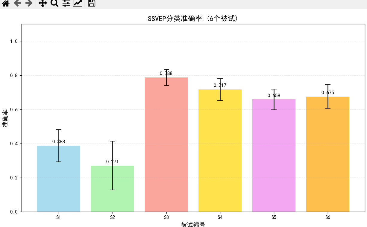
    #绘制所有被试平均准确率柱状图
    # 绘制柱状图
    plt.figure(figsize=(10, 6))

    # 创建柱状图位置
    x_pos = np.arange(len(subject_nums))

    # 绘制柱状图
    bars = plt.bar(x_pos, avg_acc_list, yerr=std_acc_list,
                   capsize=5, alpha=0.7, color=['skyblue', 'lightgreen', 'salmon',
                                                'gold', 'violet', 'orange'])

    # 添加准确率数值标签
    for bar, acc in zip(bars, avg_acc_list):
        height = bar.get_height()
        plt.text(bar.get_x() + bar.get_width() / 2., height + 0.01,
                 f'{acc:.3f}', ha='center', va='bottom')

    # 设置图表标题和标签
    plt.title('SSVEP分类准确率 (6个被试)', fontsize=14, fontweight='bold')
    plt.xlabel('被试编号', fontsize=12)
    plt.ylabel('准确率', fontsize=12)
    plt.xticks(x_pos, subject_nums)

    # 设置y轴范围（根据实际准确率调整）
    plt.ylim([0, 1.1])  # 准确率通常在0-1之间，留出一些空间

    # 添加网格线
    plt.grid(axis='y', alpha=0.3, linestyle='--')

    plt.tight_layout()
    plt.show()

4.训练的结果

5.项目链接：项目里包含了6个被试的数据

通过网盘分享的文件：CNN训练清华脑电数据
链接: https://pan.baidu.com/s/1EdAUducbRi3lgRkQMfV7vg?pwd=gq36 提取码: gq36 

项目里包含了6个被试的数据，文件稍大