基于阿里天池比赛-证券数据可视化分析（算法大赛-天池大赛-阿里云的赛制）。文章介绍当数据有明确出现date（时间），close（收盘价），open（开盘价），high（当天最高成交价），low（最低成交价），vol（交易数），amount（总金额）等数据时，我们可以采用K线可视化进行数据探索。

我们以sh_index.csv 沪市指数为例：

1.数据预处理

导入数据后，我们发现date列下的数值是int64类型（19901219），但我们希望是datetime64类型（1990-12-19）。

df_sh['date'] = pd.to_datetime(df_sh['date'],format="%Y%m%d")

df_sh是导入的原始数据，对date列处理，用pd.to_datetime。

2.K line

为了更好的展示数据，我们取2000年之后的数据。我们例子讨论（时间-收盘价）关联。出现了时间，我们一般用时序图展示。

sta_sh = df_sh[df_sh.date.dt.year > 2000]

由于date下是datetime类型，我们要取它的年份对比，用df_sh.date.dt.year取年份。

可视化，基于日，星期，月份可视化：

plt.figure(figsize=(20,14))
plt.suptitle('sh k line',fontsize=20)

plt.subplot(311)
plt.plot(sta_sh['date'],sta_sh['close'])
plt.xlabel('day')
plt.ylabel('close')
plt.title('day k-line')

plt.subplot(312)
sta_sh_week = sta_sh.resample('W-MON',on='date').agg({
    'open':'first',
    'high':'max',
    'low':'min',
    'close':'last',
    'vol':'sum',
    'amount':'sum'
})
plt.plot(sta_sh_week['close'])
plt.xlabel('week')
plt.ylabel('close')
plt.title('week k-line')

plt.subplot(313)
sta_sh_week = sta_sh.resample('M',on='date').agg({
    'open':'first',
    'high':'max',
    'low':'min',
    'close':'last',
    'vol':'sum',
    'amount':'sum'
})
plt.plot(sta_sh_week['close'])
plt.xlabel('month')
plt.ylabel('close')
plt.title('month k-line')

plt.show()

在sta_sh.resample(X,on='date')，X是'W-MON'（星期）；'M'（月）。用类似这种格式，我们可以更方便地展示数据。

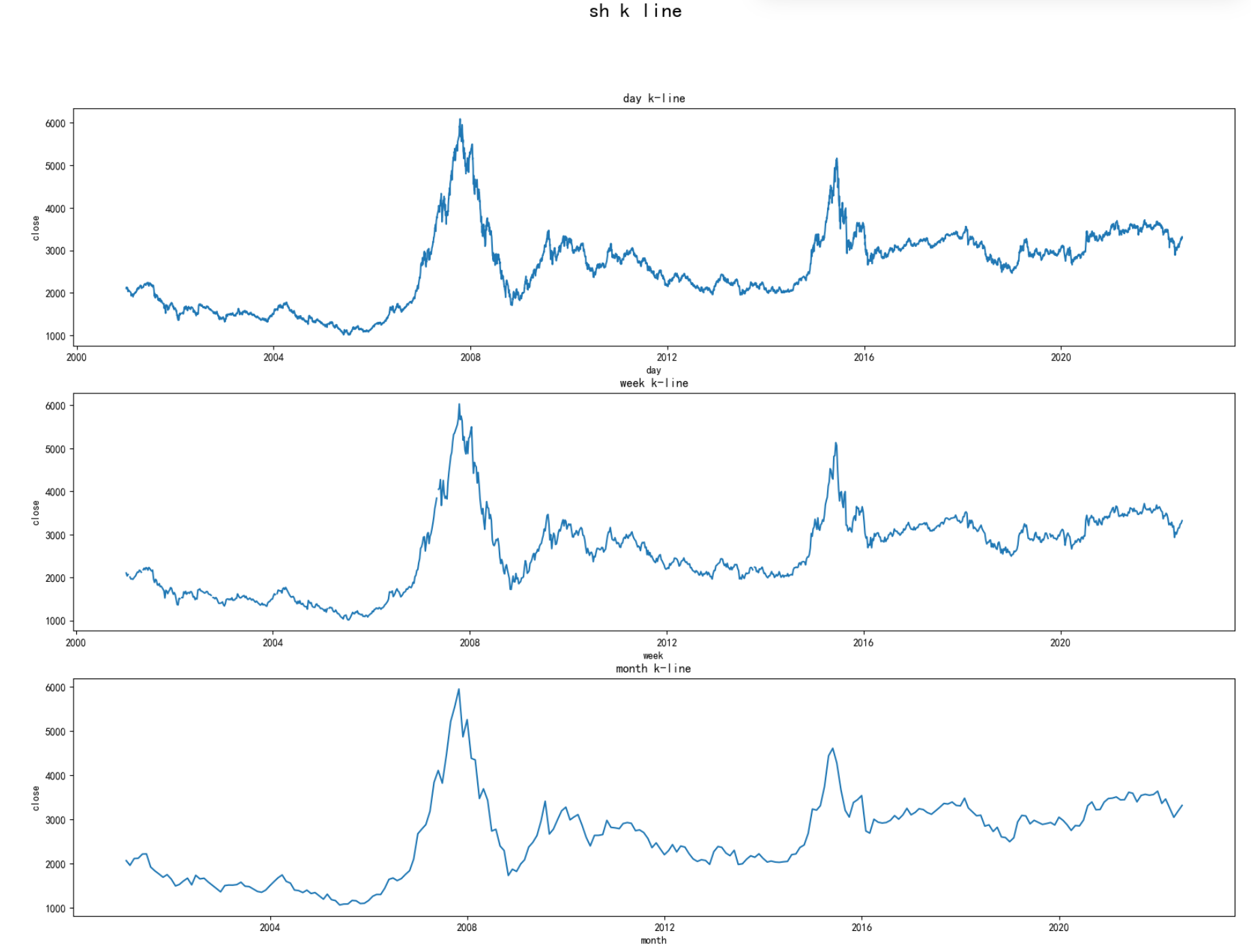
我们还可以通过改变dateframe的索引，默认是数值，我们可以将date列变成索引。

sta_sh.set_index('date',inplace=True)

成为索引后，我们可以直接用resample进行方便操作。

sta_sh_Q = sta_sh.resample('Q-DEC').mean()
sta_sh_year = sta_sh.resample('A-DEC').mean()

我们可以看一下sta_sh_Q

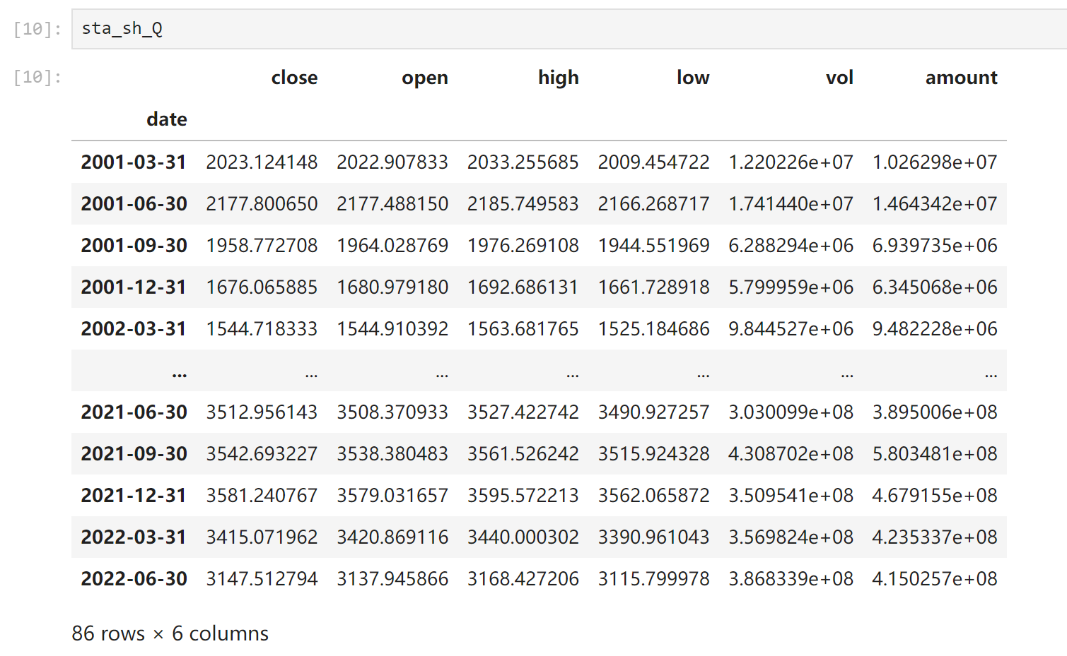
'Q-DEC'是针对季度来操作，'A-DEC'是针对年份；然后再做均值。

对close列可视化：

sta_sh.set_index('date',inplace=True)
sta_sh_Q = sta_sh.resample('Q-DEC').mean()
sta_sh_year = sta_sh.resample('A-DEC').mean()

plt.figure(figsize=(15,7))
plt.suptitle('sh mean stats',fontsize=20)
plt.subplot(221)
plt.plot(sta_sh_Q['close'],'-',label='Quarter')
plt.legend()

plt.subplot(222)
plt.plot(sta_sh_year.close,'-',label='Year')
plt.legend()

plt.show()

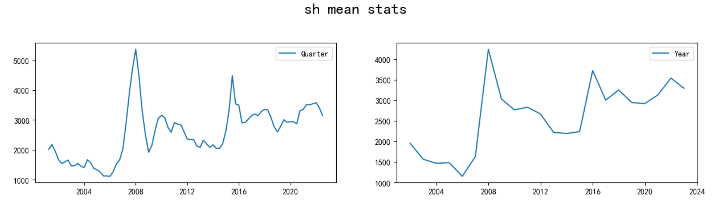
x轴是默认的索引（这个数据下就是数据了），y是close数值。

3.Mplfinance蜡烛图

sh_index_2020 = sh_index[sh_index.date.dt.year==2020]
sh_index_2020.set_index('date',inplace=True)
sh_index_2020.rename(columns={'vol':'volume'},inplace=True)
mpf.plot(
    sh_index_2020,
    type='candle',
    ylabel='price',
    style='charles',
    title='sh_index in 2020',
    mav=(5,10,30),
    volume=True,
    figratio=(5,3),
    ylabel_lower='vol'
)

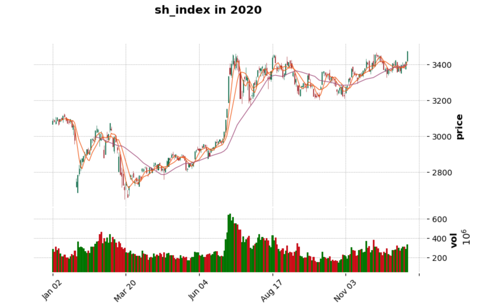
我们需要安装mplfinance库，我们一般取某一年的数据去分析，这里选择2020年，mpf中约定俗成对vol（成交量）进行有命名。同时，我们仍然要将date作为索引。其他的都是一些可变的参数了，大家可以查查大模型。

还有很多不足，大家相互学习，共同进步！