---

前言

本文主要介绍深度学习的基础内容。

---

一、torch是什么？

torch是PyTorch这个 Python 机器学习框架的核心模块：
专门为深度学习 / 机器学习设计的 “升级版 NumPy”
提供了高性能的张量（Tensor）运算、自动求导、GPU 加速等核心功能，是目前业界最主流的深度学习框架之一

二、使用步骤

1.引入库

代码如下）：

import torch
import matplotlib.pyplot as plt
import random

2.创建一个create_data函数

用来生成对应的数据：

def create_data(w, b, data_num):  # 生成数据
    x = torch.normal(0, 1, (data_num, len(w)))
    y = torch.matmul(x, w) + b

    noise = torch.normal(0, 0.01, y.shape)  # 噪声加到y上

    y += noise

    return x, y

生成矩阵x：服从均值为0，方差为1的正态分布，形状为500*4
生成带噪声的矩阵y：首先计算矩阵x与矩阵w的乘积+偏差b，再对其噪声化

---

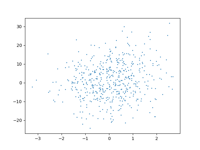
3.查看生成的数据

num = 500

true_w = torch.tensor([8.12, 2, 2, 4]) #给定权重
true_b = torch.tensor(1.1)  #给定偏差

X, Y = create_data(true_w, true_b, num)

plt.scatter(X[:, 2], Y, 1)  #此处取的第3列
plt.show()

4.按批次取数据

def data_provider(data, label, batchesize):
    length = len(label)
    indices = list(range(length))
    random.shuffle(indices)

    for each in range(0, length, batchesize):
        get_indices = indices[each: each + batchesize]
        get_data = data[get_indices]
        get_label = label[get_indices]

        yield get_data, get_label

5.定义模型

def fun(x, w, b):
    pred_y = torch.matmul(x, w) + b
    return pred_y

6.计算损失函数

def maeLoss(pre_y, y):
    return torch.sum(abs(pre_y - y)) / len(y)

7.定义随机梯度下降

def sgd(paras, lr):
    with torch.no_grad():
        for para in paras:
            para -= para.grad * lr
            para.grad.zero_()

---

8.测试

lr = 0.03  # 学习率
batchsize = 16
w_0 = torch.normal(0, 0.01, true_w.shape, requires_grad=True)
b_0 = torch.tensor(0.01, requires_grad=True)

print(w_0, b_0)

tensor([-0.0052, -0.0188, -0.0033, 0.0043], requires_grad=True) tensor(0.0100, requires_grad=True)

---

# 训练次数
epochs = 50

for epoch in range(epochs):
    data_loss = 0  # 统计每一轮loss值
    for batch_x, batch_y in data_provider(X, Y, batchsize):
        pred_y = fun(batch_x, w_0, b_0)  # 取一批数据计算预测的y
        loss = maeLoss(pred_y, batch_y)
        loss.backward()  # 梯度回传
        sgd([w_0, b_0], lr)  # 更新模型
        data_loss += loss

    print("epoch %03d: loss: %.6f" % (epoch, data_loss))

print("真实的函数值是", true_w, true_b)
print("深度训练得到的参数值是", w_0, b_0)

真实的函数值是 tensor([8.1200, 2.0000, 2.0000, 4.0000]) tensor(1.1000)
深度训练得到的参数值是 tensor([8.1322, 2.0244, 2.0072, 3.9942], requires_grad=True) tensor(1.1200, requires_grad=True)

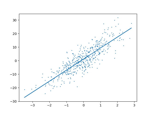
9.画图

idx = 0
plt.plot(X[:, idx].detach().numpy(), X[:, idx].detach().numpy() * w_0[idx].detach().numpy() + b_0.detach().numpy())
plt.scatter(X[:, idx], Y, 1)
plt.show()