参数初始化

均匀分布初始化

权重参数初始化从区间均匀随机取值。即在(-1/√d, +1/√d)均匀分布中生成当前神经元的权重，其中d为每个神经元的输入数量。

import torch
import torch.nn as nn

torch.manual_seed(40)


def test01():
    linear = nn.Linear(5, 3)
    nn.init.uniform_(
        tensor=linear.weight,
        a=0.0,
        b=1.0,
    )
    print(linear.weight.data)


test01()

tensor([[0.6779, 0.0173, 0.1203, 0.1363, 0.8089],
        [0.8229, 0.3759, 0.0295, 0.4132, 0.0791],
        [0.0489, 0.9287, 0.4924, 0.8416, 0.1756]])

正态分布初始化

随机初始化从均值为0，标准差是1的高斯分布中取样，使用一些很小的值对参数W进行初始化。

import torch
import torch.nn as nn

torch.manual_seed(40)


def test02():
    linear = nn.Linear(5, 3)
    nn.init.normal_(linear.weight, mean=0, std=1)
    print(linear.weight.data)


test02()

tensor([[-0.4778,  0.9635,  1.0699, -0.1470, -0.4221],
        [-0.3340, -1.3286,  0.9798,  1.0087, -1.7466],
        [ 0.3339,  1.3638,  1.1793,  0.8641, -1.5166]])

全0初始化

将神经网络中的所有权重参数初始化为0。

import torch
import torch.nn.functional as F
import torch.nn as nn

torch.manual_seed(40)



def test03():
    linear = nn.Linear(5, 3)
    nn.init.zeros_(linear.weight)
    print(linear.weight.data)


test03()

tensor([[0., 0., 0., 0., 0.],
        [0., 0., 0., 0., 0.],
        [0., 0., 0., 0., 0.]])

全1初始化

将神经网络中的所有权重参数初始化为1。

import torch
import torch.nn.functional as F
import torch.nn as nn

torch.manual_seed(40)


def test04():
    linear = nn.Linear(5, 3)
    nn.init.ones_(linear.weight)
    print(linear.weight.data)


test04()

tensor([[1., 1., 1., 1., 1.],
        [1., 1., 1., 1., 1.],
        [1., 1., 1., 1., 1.]])

固定值初始化

将神经网络中的所有权重参数初始化为某个固定值。

import torch
import torch.nn.functional as F
import torch.nn as nn

torch.manual_seed(40)


def test05():
    linear = nn.Linear(5, 3)
    nn.init.constant_(linear.weight, 5)
    print(linear.weight.data)


test05()

tensor([[5., 5., 5., 5., 5.],
        [5., 5., 5., 5., 5.],
        [5., 5., 5., 5., 5.]])

kaiming 初始化，也叫做HE 初始化

HE 初始化分为正态分布的HE 初始化、均匀分布的HE 初始化。

正态化的he初始化， 均值为 0、标准差为stddev = sqrt(2 / fan_in)，值绝大多数落在 [-3stddev, 3stddev] 区间内。

均匀分布的he初始化，它从[-limit，limit] 中的均匀分布中抽取样本, limit是 sqrt(6 / fan_in)

fan_in 输入神经元的个数。

import torch
import torch.nn.functional as F
import torch.nn as nn

torch.manual_seed(40)


def test06():
    # kaiming正态分布初始化
    linear = nn.Linear(5, 3)
    nn.init.kaiming_normal_(linear.weight)
    print(linear.weight.data)
    # kaiming均匀分布初始化
    linear = nn.Linear(5, 3)
    nn.init.kaiming_uniform_(linear.weight)
    print(linear.weight.data)


test06()

tensor([[ 0.4088, -1.0591,  0.4997, -0.4519,  0.0120],
        [-0.1373,  0.5314, -0.8153, -0.4597, -0.3746],
        [ 0.7623,  0.0659, -0.3816, -0.9031,  0.1621]])
tensor([[ 0.4260, -0.5625, -0.9473, -0.9170, -0.6304],
        [ 0.5598,  0.5249, -0.9120, -0.8568, -0.9133],
        [ 0.4550, -0.0920,  0.1418,  0.0992,  0.7793]])

xavier 初始化，也叫做Glorot初始化

该方法也有两种，一种是正态分布的xavier初始化、一种是均匀分布的xavier 初始化。

正态化的Xavier初始化， 均值为 0、标准差为stddev = sqrt(2 / (fan_in + fan_out))，值绝大多数落在 [-3stddev, 3stddev] 区间内。

均匀分布的Xavier初始化，[-limit，limit] 中的均匀分布中抽取样本, limit 是 sqrt(6 / (fan_in + fan_out))。

fan_in 是输入神经元的个数，fan_out 是输出的神经元个数。

import torch
import torch.nn.functional as F
import torch.nn as nn

torch.manual_seed(40)


def test07():
    # xavier正态分布初始化
    linear = nn.Linear(5, 3)
    nn.init.xavier_normal_(linear.weight)
    print(linear.weight.data)
    # xavier均匀分布初始化
    linear = nn.Linear(5, 3)
    nn.init.xavier_uniform_(linear.weight)
    print(linear.weight.data)


test07()

tensor([[ 0.8132, -0.0745, -0.2696,  0.1094, -0.4667],
        [-0.0538,  0.1478, -0.1500, -0.1905, -0.3753],
        [-0.7975,  0.2913,  0.0392,  0.1245,  0.1830]])
tensor([[ 0.6763,  0.0562,  0.6092,  0.7034,  0.8327],
        [-0.1684,  0.0137,  0.7739, -0.1965,  0.6781],
        [-0.3610, -0.2906,  0.8220, -0.6182, -0.3569]])

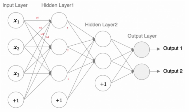
神经网络搭建和参数计算

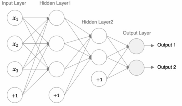
编码设计如下:
1.第1个隐藏层:权重初始化采用标准化的xavier初始化激活函数使用sigmoid。

2.第2个隐藏层:权重初始化采用标准化的He初始化激活函数采用relu。

3.out输出层线性层假若二分类，采用softmax做数据归一化。

import torch
import torch.nn as nn
# 计算模型参数,查看模型结构, pip install torchsummary
from torchsummary import summary


# 创建神经网络模型类
class Model(nn.Module):
    # 初始化属性值
    def __init__(self):
        # 调用父类的初始化属性值
        super(Model, self).__init__()

        # 创建第一个隐藏层模型, 3个输入特征,3个输出特征
        self.linear1 = nn.Linear(3, 3)
        # 初始化权
        nn.init.xavier_normal_(self.linear1.weight)

        # 创建第二个隐藏层模型, 3个输入特征(上一层的输出特征),2个输出特征
        self.linear2 = nn.Linear(3, 2)
        # 初始化权重
        nn.init.kaiming_normal_(self.linear2.weight)

        # 创建输出层模型
        self.out = nn.Linear(2, 2)

    # 创建前向传播方法,自动执行forward()方法
    def forward(self, x):
        # 数据经过第一个线性层
        x = self.linear1(x)
        # 使用sigmoid激活函数
        x = torch.sigmoid(x)

        # 数据经过第二个线性层
        x = self.linear2(x)
        # 使用relu激活函数
        x = torch.relu(x)

        # 数据经过输出层
        x = self.out(x)
        # 使用softmax激活函数
        # dim=-1:每一维度行数据相加为1
        x = torch.softmax(x, dim=-1)

        return x


if __name__ == "__main__":
    # 实例化model对象
    my_model = Model()
    # 随机产生数据
    my_data = torch.randn(5, 3)
    print("mydata shape", my_data.shape)
    # 数据经过神经网络模型训练
    output = my_model(my_data)
    print("output shape-->", output.shape)
    # 计算模型参数
    # 计算每层每个神经元的w和b个数总和
    summary(my_model, input_size=(3,), batch_size=5)
    # 查看模型参数
    print("======查看模型参数w和b======")
    for name, parameter in my_model.named_parameters():
        print(name, parameter)

mydata shape torch.Size([5, 3])
output shape--> torch.Size([5, 2])
----------------------------------------------------------------
        Layer (type)               Output Shape         Param #
================================================================
            Linear-1                     [5, 3]              12
            Linear-2                     [5, 2]               8
            Linear-3                     [5, 2]               6
================================================================
Total params: 26
Trainable params: 26
Non-trainable params: 0
----------------------------------------------------------------
Input size (MB): 0.00
Forward/backward pass size (MB): 0.00
Params size (MB): 0.00
Estimated Total Size (MB): 0.00
----------------------------------------------------------------
======查看模型参数w和b======
linear1.weight Parameter containing:
tensor([[-6.7921e-01, -8.9048e-04, -1.6005e-01],
        [-3.8197e-01,  8.6354e-01, -1.1468e+00],
        [ 5.2889e-02, -7.4933e-02,  1.9173e-01]], requires_grad=True)
linear1.bias Parameter containing:
tensor([-0.0769, -0.3757, -0.0714], requires_grad=True)
linear2.weight Parameter containing:
tensor([[ 0.7111, -0.3630,  0.6903],
        [ 0.5848,  1.1082,  0.7090]], requires_grad=True)
linear2.bias Parameter containing:
tensor([-0.2732,  0.3150], requires_grad=True)
out.weight Parameter containing:
tensor([[-0.5128,  0.1292],
        [ 0.5511, -0.1931]], requires_grad=True)
out.bias Parameter containing:
tensor([0.0501, 0.1868], requires_grad=True)

模型参数的计算:

1. 以第一个隐层为例：该隐层有3个神经元，每个神经元的参数为：4个（w1,w2,w3,b1），所以一共用3x4=12个参数。

2. 输入数据和网络权重是两个不同的事儿！对于初学者理解这一点十分重要，要分得清。

神经网络的优缺点

1.优点

Ø 精度⾼，性能优于其他的机器学习⽅法，甚⾄在某些领域超过了⼈类

Ø 可以近似任意的⾮线性函数随之计算机硬件的发展

Ø 近年来在学界和业界受到了热捧，有⼤量的框架和库可供调。

2.缺点

Ø ⿊箱，很难解释模型是怎么⼯作的

Ø 训练时间⻓，需要⼤量的计算⼒

Ø ⽹络结构复杂，需要调整超参数

Ø ⼩数据集上表现不佳，容易发⽣过拟合