一、PyTorch框架介绍

1.1 PyTorch概述

PyTorch是由Facebook人工智能研究院（FAIR）开发的开源深度学习框架，以其动态计算图、直观的API设计和强大的GPU加速能力而闻名。

1.2 核心特性

特性	说明	优势
动态计算图​	运行时构建计算图	灵活调试，支持动态网络结构
张量计算​	类似NumPy的接口	易于学习，支持GPU加速
自动微分​	Autograd系统	自动计算梯度，简化反向传播
模块化设计​	nn.Module基类	代码复用，易于构建复杂网络
丰富的生态系统​	torchvision、torchaudio等	提供预训练模型、数据集和工具

1.3 PyTorch和CUDA关系

CUDA（Compute Unified Device Architecture）是NVIDIA推出的通用并行计算架构，允许开发人员使用NVIDIA GPU进行通用计算。

# CUDA的核心能力：
1. 并行计算: GPU拥有数千个计算核心
2. 内存层次: 全局内存、共享内存、寄存器
3. 编程模型: 线程层次结构（线程→线程块→网格）

维度	说明	关系描述
架构关系​	PyTorch是深度学习框架，CUDA是计算平台	PyTorch在CUDA之上构建GPU加速能力
依赖关系​	PyTorch可选依赖CUDA	可以安装CPU-only或CUDA版本
调用关系​	PyTorch调用CUDA API	通过CUDA Runtime API和cuDNN加速计算
性能关系​	CUDA提供硬件加速	PyTorch通过CUDA实现10-100倍性能提升

 

二、VGG-16模型详解

2.1 VGG网络发展背景

VGG（Visual Geometry Group）网络由牛津大学视觉几何组于2014年提出，在ImageNet图像分类竞赛中取得了优异成绩。

2.2 VGG-16网络架构

2.2.1 整体结构

输入: 224×224×3 RGB图像
↓
卷积层组1: 2个3×3卷积(64通道) → ReLU → 2×2最大池化
↓
卷积层组2: 2个3×3卷积(128通道) → ReLU → 2×2最大池化
↓
卷积层组3: 3个3×3卷积(256通道) → ReLU → 2×2最大池化
↓
卷积层组4: 3个3×3卷积(512通道) → ReLU → 2×2最大池化
↓
卷积层组5: 3个3×3卷积(512通道) → ReLU → 2×2最大池化
↓
展平: 7×7×512 = 25088维向量
↓
全连接层1: 4096神经元 → ReLU → Dropout(0.5)
↓
全连接层2: 4096神经元 → ReLU → Dropout(0.5)
↓
全连接层3: 1000神经元（对应ImageNet 1000类）
↓
输出: 1000维概率分布

2.2.2 关键设计特点

1. 小卷积核策略

   • 全部使用3×3卷积核

   • 两个3×3卷积层相当于一个5×5的感受野

   • 三个3×3卷积层相当于一个7×7的感受野

   • 优势：减少参数数量，增加非线性激活

2. 参数计算示例

   # 3×3卷积参数计算
   # 输入通道: C_in, 输出通道: C_out
   # 参数数量 = C_in × C_out × 3 × 3 + C_out (偏置)
   
   # 示例: 第一层卷积
   # 输入: 3通道, 输出: 64通道
   # 参数 = 3 × 64 × 3 × 3 + 64 = 1,792
   
   # 对比: 7×7卷积
   # 参数 = 3 × 64 × 7 × 7 + 64 = 9,472

3. 池化策略

   • 使用2×2最大池化，步长为2

   • 每次池化后特征图尺寸减半

   • 共5次池化：224→112→56→28→14→7

2.3 VGG-16参数统计

层类型	层数	参数数量	占比
卷积层	13	14,714,688	约10.6%
全连接层	3	123,650,048	约89.4%
总计​	16​	138,364,736​	100%​

2.4 VGG变体比较

模型	卷积层数	全连接层数	总层数	参数量
VGG-11	8	3	11	约1.33亿
VGG-13	10	3	13	约1.33亿
VGG-16​	13​	3​	16​	约1.38亿​
VGG-19	16	3	19	约1.44亿

三、 VGG-16模型载入&可视化

Jupyter中的内嵌显示工具：

工具	Jupyter内嵌支持	具体实现方式	显示效果
torchviz​	✅ 支持​	使用IPython.display.display(dot)直接显示SVG图形	静态SVG图，快速查看计算图，可缩放查看细节
TensorBoard​	✅ 支持​	使用%load_ext tensorboard和%tensorboard --logdir logs魔法命令	内嵌iframe，完整TensorBoard界面，控训练过程和查看模型图

3.1 torchviz方案

# 导入必要的库
import os
import torch
from torchvision import models
from torchviz import make_dot
from IPython.display import display

# ========== 第一部分：加载预训练的VGG-16模型 ==========

# 生成VGG-16模型的实例
# use_pretrained = True 表示使用在ImageNet数据集上预训练的权重参数
# 第一次运行时会从网络下载约500MB的模型权重文件
# 在大多数情况下，下载的模型权重文件保存在以下目录中：
# Linux/Unix: ~/.cache/torch/hub/checkpoints/
# Windows: C:\\Users\\<用户名>\\.cache\\torch\\hub\\checkpoints\\
# macOS: ~/.cache/torch/hub/checkpoints/
use_pretrained = True
net = models.vgg16(pretrained=use_pretrained)

# 将模型设置为评估模式（推测模式）
# eval()的作用：
# 1. 关闭Dropout层（训练时用于正则化，推理时不需要）
# 2. 固定BatchNorm层的均值和方差（使用训练时计算的统计量）
# 3. 提高推理速度和一致性
net.eval()

# 输出模型的网络结构
# 打印显示VGG-16的完整层次结构：
# - features模块：13个卷积层 + 5个最大池化层
# - classifier模块：3个全连接层 + 2个Dropout层
print("VGG-16模型结构:")
print("=" * 60)
print(net)
print("=" * 60)

# ========== 第二部分：准备保存目录 ==========

# 创建保存可视化结果的目录
save_dir = "./vgg16_visualization"
# os.makedirs创建目录，exist_ok=True表示如果目录已存在不会报错
os.makedirs(save_dir, exist_ok=True)
print(f"可视化结果将保存到: {save_dir}")

# ========== 第三部分：准备输入数据 ==========

# 创建虚拟输入张量
# torch.randn(1, 3, 224, 224) 创建一个符合标准正态分布的随机张量：
# - 1: batch_size（批量大小），一次处理1张图片
# - 3: channels（通道数），对应RGB三个颜色通道
# - 224, 224: height和width（高度和宽度），VGG-16的标准输入尺寸
dummy_input = torch.randn(1, 3, 224, 224)
print(f"输入张量形状: {dummy_input.shape}")

# ========== 第四部分：开始可视化流程 ==========

print("\n🚀 开始可视化VGG-16模型...")
print("=" * 50)

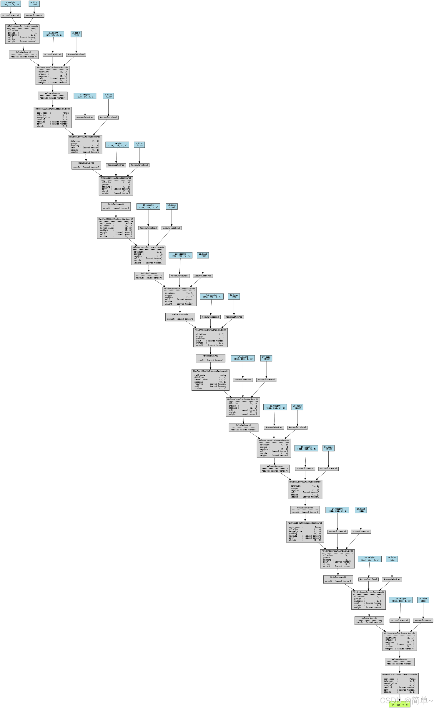
# 步骤1：生成完整计算图（简化版）
print("\n1. 生成完整计算图（简化）...")

# 使用torch.no_grad()上下文管理器
# 作用：不计算梯度，节省内存，提高前向传播速度
with torch.no_grad():
    # 前向传播，获取模型输出
    # 输出形状应为[1, 1000]，对应ImageNet的1000个类别
    output = net(dummy_input)
    print(f"模型输出形状: {output.shape}")

# 生成简化版计算图
# make_dot()参数说明：
# - output: 模型的输出张量
# - params: 要可视化的模型参数
#   dict(net.named_parameters())获取所有可学习参数的字典
simple_dot = make_dot(output, params=dict(net.named_parameters()))

# 设置图形属性
# - rankdir='LR': 从左到右布局（Left to Right）
# - size='20,20': 图形尺寸为20x20英寸
simple_dot.attr(rankdir='LR', size='20,20')

# 保存为PNG图片
# 参数说明：
# - os.path.join(save_dir, "vgg16_simple"): 生成完整文件路径
# - format="png": 保存为PNG格式
# - cleanup=True: 保存后清理中间文件
simple_dot.render(os.path.join(save_dir, "vgg16_simple"), format="png", cleanup=True)

# 在Jupyter中直接显示SVG图形
# display()函数会将图形内嵌在单元格中
display(simple_dot)
print("✅ 简化版计算图已生成并显示")

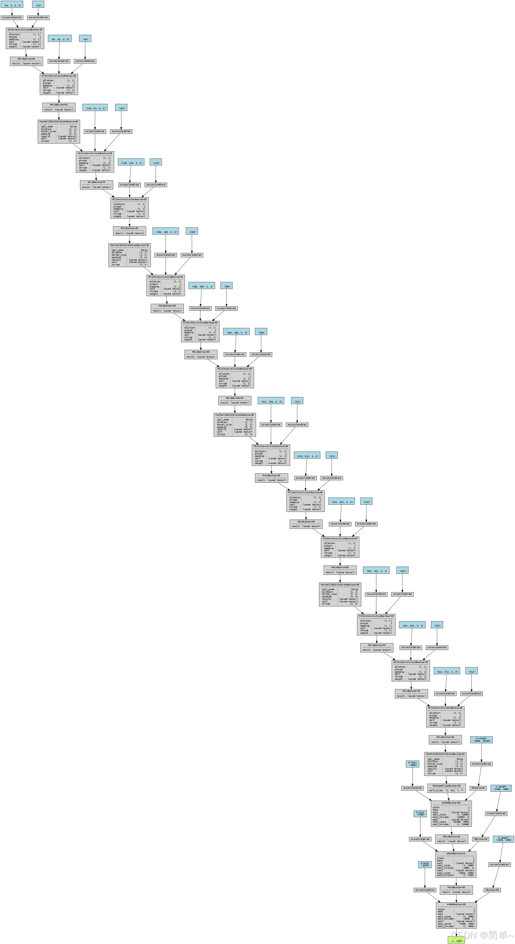
# 步骤2：生成详细计算图
print("\n2. 生成详细计算图...")

# 生成详细版计算图
# 额外参数说明：
# - show_attrs=True: 显示节点的属性信息（如卷积核大小、步长等）
# - show_saved=True: 显示在计算图中保存的中间张量
detailed_dot = make_dot(output, 
                        params=dict(net.named_parameters()),
                        show_attrs=True,
                        show_saved=True)

# 设置详细图的属性
# - rankdir='TB': 从上到下布局（Top to Bottom），适合显示深层网络
# - size='30,50': 更大的图形尺寸，因为详细图更复杂
detailed_dot.attr(rankdir='TB', size='30,50')

# 保存为SVG格式（矢量图）
# SVG格式的优点：
# 1. 矢量图形，可无限放大不失真
# 2. 适合查看复杂图形的细节
# 3. 文件大小相对较小
detailed_dot.render(os.path.join(save_dir, "vgg16_detailed"), format="svg", cleanup=True)

# 在Jupyter中显示详细计算图
display(detailed_dot)
print("✅ 详细版计算图已生成并显示")

# 步骤3：分段可视化
print("\n3. 分段可视化...")

# 3.1 可视化特征提取器（features模块）
print("\n  3.1 可视化特征提取器（features模块）...")

# 提取特征提取器的输出
# net.features包含：
# - 13个卷积层（Conv2d）
# - 13个ReLU激活函数
# - 5个最大池化层（MaxPool2d）
# 输入: 224×224×3 → 输出: 7×7×512
features_output = net.features(dummy_input)
print(f"    特征提取器输出形状: {features_output.shape}")

# 生成特征提取器的计算图
features_dot = make_dot(features_output, 
                        params=dict(net.features.named_parameters()),
                        show_attrs=True)

# 保存特征提取器图
features_dot.render(os.path.join(save_dir, "vgg16_features"), format="png", cleanup=True)

# 显示特征提取器图
display(features_dot)
print("    ✅ 特征提取器图已生成并显示")

# 3.2 可视化分类器（classifier模块）
print("\n  3.2 可视化分类器（classifier模块）...")

# 展平特征提取器的输出
# 原始形状: [1, 512, 7, 7]
# 展平后: [1, 512 * 7 * 7] = [1, 25088]
# 全连接层需要二维输入: [batch_size, features]
features_flattened = torch.flatten(features_output, 1)
print(f"    展平后的特征形状: {features_flattened.shape}")

# 分类器前向传播
# net.classifier包含：
# - 第一个全连接层: 25088 → 4096
# - Dropout层（p=0.5）
# - 第二个全连接层: 4096 → 4096
# - Dropout层（p=0.5）
# - 第三个全连接层: 4096 → 1000
classifier_output = net.classifier(features_flattened)
print(f"    分类器输出形状: {classifier_output.shape}")

# 生成分类器的计算图
classifier_dot = make_dot(classifier_output, 
                          params=dict(net.classifier.named_parameters()),
                          show_attrs=True)

# 保存分类器图
classifier_dot.render(os.path.join(save_dir, "vgg16_classifier"), format="png", cleanup=True)

# 显示分类器图
display(classifier_dot)
print("    ✅ 分类器图已生成并显示")

# ========== 第五部分：结果汇总 ==========

print(f"\n✅ 可视化完成！文件保存在: {save_dir}")
print("\n生成的文件:")
print(f"  - {save_dir}/vgg16_simple.png    (简化版，PNG格式)")
print(f"  - {save_dir}/vgg16_detailed.svg  (详细版，SVG矢量图格式)")
print(f"  - {save_dir}/vgg16_features.png  (特征提取器，PNG格式)")
print(f"  - {save_dir}/vgg16_classifier.png (分类器，PNG格式)")

print("\n" + "="*50)
print("文件格式说明:")
print("="*50)
print("PNG格式: 位图格式，适合快速查看和分享")
print("SVG格式: 矢量图格式，可无限放大查看细节")
print("\n" + "="*50)
print("模型参数统计:")
print("="*50)

# 计算并显示模型参数统计
total_params = sum(p.numel() for p in net.parameters())
trainable_params = sum(p.numel() for p in net.parameters() if p.requires_grad)

print(f"总参数量: {total_params:,} 个参数")
print(f"可训练参数: {trainable_params:,} 个参数")

# 各模块参数统计
features_params = sum(p.numel() for p in net.features.parameters())
classifier_params = sum(p.numel() for p in net.classifier.parameters())

print(f"\n模块参数量分布:")
print(f"特征提取器 (features): {features_params:,} 个参数 ({features_params/total_params*100:.1f}%)")
print(f"分类器 (classifier): {classifier_params:,} 个参数 ({classifier_params/total_params*100:.1f}%)")

print("\n" + "="*50)
print("可视化工具使用提示:")
print("="*50)
print("1. SVG文件可以用浏览器或矢量图编辑器（如Inkscape）打开")
print("2. 在Jupyter中点击图片，可以在新标签页打开并缩放查看细节")
print("3. 如果图形过大，建议分段查看features和classifier模块")
print("4. 详细图包含节点属性，适合深入理解模型结构")

输出：

================================================== 

1. 生成完整计算图（简化）... 模型输出形状: torch.Size([1, 1000])

Output is truncated. View as a scrollable element or open in a text editor. Adjust cell output settings...

(1, 1000)

✅ 简化版计算图已生成并显示 

2. 生成详细计算图...

(1, 1000)

✅ 详细版计算图已生成并显示 

3. 分段可视化... 

3.1 可视化特征提取器（features模块）... 

特征提取器输出形状: torch.Size([1, 512, 7, 7])

✅ 特征提取器图已生成并显示 

3.2 可视化分类器（classifier模块）... 

展平后的特征形状: torch.Size([1, 25088]) 

分类器输出形状: torch.Size([1, 1000])

✅ 分类器图已生成并显示

✅ 可视化完成！文件保存在: ./vgg16_visualization

生成的文件:
  - ./vgg16_visualization/vgg16_simple.png    (简化版，PNG格式)
  - ./vgg16_visualization/vgg16_detailed.svg  (详细版，SVG矢量图格式)
  - ./vgg16_visualization/vgg16_features.png  (特征提取器，PNG格式)
  - ./vgg16_visualization/vgg16_classifier.png (分类器，PNG格式)

==================================================
文件格式说明:
==================================================
PNG格式: 位图格式，适合快速查看和分享
SVG格式: 矢量图格式，可无限放大查看细节

==================================================
模型参数统计:
==================================================
总参数量: 138,357,544 个参数
可训练参数: 138,357,544 个参数

模块参数量分布:
特征提取器 (features): 14,714,688 个参数 (10.6%)
分类器 (classifier): 123,642,856 个参数 (89.4%)

==================================================
可视化工具使用提示:
==================================================
1. SVG文件可以用浏览器或矢量图编辑器（如Inkscape）打开
2. 在Jupyter中点击图片，可以在新标签页打开并缩放查看细节
3. 如果图形过大，建议分段查看features和classifier模块
4. 详细图包含节点属性，适合深入理解模型结构

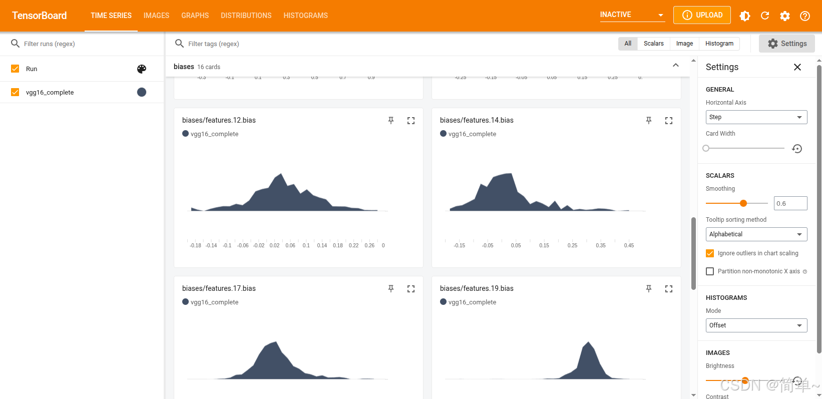
3.2 tensorboard方案

# 扩展功能：添加权重直方图和示例图片
import torch
import torchvision.models as models
import torchvision.transforms as transforms
from torch.utils.tensorboard import SummaryWriter
from PIL import Image
import requests
from io import BytesIO
import matplotlib.pyplot as plt
from torchvision.utils import make_grid  # 导入 make_grid
%matplotlib inline

# 1. 创建模型
net = models.vgg16(pretrained=True)
net.eval()

# 2. 创建 SummaryWriter
writer = SummaryWriter('runs/vgg16_complete')

# 3. 添加模型图
dummy_input = torch.randn(1, 3, 224, 224)
writer.add_graph(net, dummy_input)

# 4. 添加权重直方图
for name, param in net.named_parameters():
    if 'weight' in name:
        writer.add_histogram(f'weights/{name}', param, 0)
    if 'bias' in name:
        writer.add_histogram(f'biases/{name}', param, 0)

# 5. 加载示例图片
image_file_path = './data/goldenretriever-3724972_640.jpg'
img = Image.open(image_file_path)

# 预处理
transform = transforms.Compose([
    transforms.Resize(256),
    transforms.CenterCrop(224),
    transforms.ToTensor(),
    transforms.Normalize(mean=[0.485, 0.456, 0.406], std=[0.229, 0.224, 0.225]),
])
input_tensor = transform(img).unsqueeze(0)

# 添加输入图片到 TensorBoard
img_tensor = transform(img)
writer.add_image('input/cat_image', img_tensor, 0)

# 6. 注册钩子来获取中间层特征
features = {}
def get_features(name):
    def hook(model, input, output):
        features[name] = output.detach()
    return hook

# 注册钩子到前几个卷积层
layers_to_visualize = ['features.0', 'features.2', 'features.5']
for layer_name in layers_to_visualize:
    layer = dict(net.features.named_children())[layer_name.split('.')[-1]]
    layer.register_forward_hook(get_features(layer_name))

# 前向传播
with torch.no_grad():
    output = net(input_tensor)

# 7. 添加特征图到 TensorBoard ✅ 修正此处
for layer_name, feature in features.items():
    # 取第 1 个样本的前 8 个通道
    feature_slice = feature[0, 0:8, :, :]  # (8, H, W)
    
    # 使用 make_grid 拼接成网格显示
    grid = make_grid(feature_slice.unsqueeze(1),  # (8, 1, H, W)
                     nrow=4,                       # 每行 4 个
                     normalize=True,               # 归一化到 [0, 1]
                     scale_each=True)              # 每个通道单独归一化
    
    writer.add_image(f'features/{layer_name}/grid', grid, 0)

# 8. 关闭 writer
writer.close()

print("所有可视化数据已写入 TensorBoard！")
# 加载 TensorBoard 扩展
%load_ext tensorboard

# 启动 TensorBoard，指定日志目录
%tensorboard --logdir runs

输出：

直接在浏览器中访问：http://localhost:6006

3.3 VGG16网络结构图

VGG16 结构核心特点：

1.  深度统一：整个网络由13个卷积层和3个全连接层构成，共16层（故名VGG16）。
2.  小卷积核：全部使用3×3的小型卷积核，通过堆叠来替代更大的感受野（如2个3x3卷积等价于1个5x5卷积）。
3.  规律堆叠：卷积层通常以2-4个为一组，每组后接一个2×2最大池化进行下采样，空间尺寸减半，通道数翻倍（最后一组除外）。
4.  通道数变化：64 → 128 → 256 → 512 → 512，体现了特征图数量（通道深度）逐渐增加，而尺寸逐渐减小的过程。
5.  全连接分类：最后通过3个全连接层将提取的7x7x512=25088维特征映射到1000个类别的概率。

这个结构因其简洁、规整和深度，成为计算机视觉领域里程碑式的经典网络。

四、VGG-16的优势与局限

4.1 优势

1. 结构简单统一

   • 全部使用3×3卷积核

   • 每层结构相似，易于理解和实现

2. 性能优秀

   • 在ImageNet上达到92.7%的top-5准确率

   • 特征提取能力强

3. 迁移学习效果好

   • 预训练权重广泛可用

   • 适用于各种计算机视觉任务

4.2 局限性

1. 参数量大

   • 全连接层参数过多（约1.23亿）

   • 存储和计算成本高

2. 训练困难

   • 需要大量数据和计算资源

   • 训练时间较长

3. 内存占用高

   • 中间特征图占用大量内存

   • 不适合移动设备部署

五、实际应用示例

5.1 请大橘😺

5.2 VGG预测图片分类

# 导入必要的包
import numpy as np
import json
from PIL import Image
import matplotlib.pyplot as plt
%matplotlib inline

import torch
import torchvision
from torchvision import models, transforms

# ========== 第一部分：定义图片预处理类 ==========

class BaseTransform():
    """
    调整图片的尺寸，并对颜色进行规范化。
    这是深度学习模型输入图片前的标准预处理步骤。

    Attributes
    ----------
    resize : int
        指定调整尺寸后图片的大小
    mean : (R, G, B)
        各个颜色通道的平均值（ImageNet数据集的平均颜色）
    std : (R, G, B)
        各个颜色通道的标准偏差（ImageNet数据集的标准差）
    """

    def __init__(self, resize, mean, std):
        """
        初始化预处理流水线
        
        参数:
        - resize: 目标图片尺寸（VGG-16使用224x224）
        - mean: 每个颜色通道的均值，用于归一化
        - std: 每个颜色通道的标准差，用于归一化
        """
        # 使用transforms.Compose组合多个预处理操作
        self.base_transform = transforms.Compose([
            # 1. 调整图片尺寸
            transforms.Resize(resize),  # 将较短边的长度调整到resize大小，保持长宽比
            # 2. 从中心裁剪
            transforms.CenterCrop(resize),  # 从图片中央截取resize × resize大小的正方形区域
            # 3. 转换为PyTorch张量
            transforms.ToTensor(),  # 将PIL图片或numpy数组转换为torch.Tensor
            # 4. 颜色归一化
            transforms.Normalize(mean, std)  # 用均值和标准差对每个通道进行归一化
        ])

    def __call__(self, img):
        """
        使类的实例可以像函数一样调用
        
        参数:
        - img: PIL.Image对象，原始输入图片
        
        返回:
        - torch.Tensor: 预处理后的图片张量
        """
        return self.base_transform(img)

# ========== 第二部分：定义预测结果后处理类 ==========

class ILSVRCPredictor():
    """
    根据ILSVRC数据集（ImageNet挑战赛），从模型的输出结果计算出分类标签
    
    ILSVRC: ImageNet Large Scale Visual Recognition Challenge
    这是计算机视觉领域最著名的比赛，包含1000个物体类别

    Attributes
    ----------
    class_index : dictionary
        将类别索引与标签名关联起来的字典变量
        格式: {类别索引: [WordNet ID, 类别描述]}
    """

    def __init__(self, class_index):
        """
        初始化预测器
        
        参数:
        - class_index: 包含1000个ImageNet类别信息的字典
        """
        self.class_index = class_index

    def predict_max(self, out):
        """
        获得概率最大的ILSVRC分类标签名
        
        参数:
        ----------
        out : torch.Size([1, 1000])
            从VGG-16模型输出的1000个类别的概率分布
            
        返回:
        -------
        predicted_label_name : str
            预测概率最高的分类标签的名称
        """
        # 1. 从计算图中分离张量，转换为numpy数组
        # detach(): 从当前计算图中分离张量，不再跟踪梯度
        # numpy(): 转换为numpy数组
        out_numpy = out.detach().numpy()
        
        # 2. 找到概率最大的类别索引
        # np.argmax(): 返回数组中最大值的索引
        maxid = np.argmax(out_numpy)
        
        # 3. 根据索引从class_index字典中获取标签名
        # 格式: class_index[str(maxid)] = [WordNet ID, 类别描述]
        predicted_label_name = self.class_index[str(maxid)][1]
        
        return predicted_label_name

# ========== 第三部分：验证图片预处理效果 ==========

print("🚀 开始验证图片预处理效果...")
print("=" * 50)

# 1. 读取图片
image_file_path = './data/1.jpg'
try:
    # 使用PIL打开图片
    # PIL.Image.open(): 打开图片文件，返回Image对象
    # 图片格式: [高度][宽度][颜色RGB]
    img = Image.open(image_file_path)
    print(f"✅ 成功读取图片: {image_file_path}")
    print(f"   原始图片尺寸: {img.size} (宽度×高度)")
    print(f"   图片模式: {img.mode} (RGB或L等)")
except Exception as e:
    print(f"❌ 无法读取图片: {e}")
    exit()

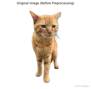
# 2. 显示处理前的图片
print("\n📸 显示原始图片...")
plt.figure(figsize=(8, 6))
plt.imshow(img)
plt.title("Original Image (Before Preprocessing)")  # 图表标题用英文
plt.axis('off')  # 不显示坐标轴
plt.show()

# 3. 同时显示预处理前后的图片
print("\n🔧 应用预处理转换...")

# 设置预处理参数（VGG-16标准参数）
resize = 224  # VGG-16的标准输入尺寸
mean = (0.485, 0.456, 0.406)  # ImageNet数据集的RGB均值
std = (0.229, 0.224, 0.225)   # ImageNet数据集的RGB标准差

print(f"   目标尺寸: {resize}x{resize}")
print(f"   均值 (R, G, B): {mean}")
print(f"   标准差 (R, G, B): {std}")

# 创建预处理实例
transform = BaseTransform(resize, mean, std)

# 应用预处理
img_transformed = transform(img)  # 输出: torch.Size([3, 224, 224])

print(f"   预处理后张量形状: {img_transformed.shape}")
print(f"   数据类型: {img_transformed.dtype}")
print(f"   取值范围: [{img_transformed.min():.3f}, {img_transformed.max():.3f}]")

# 4. 将处理后的张量转换为可显示的格式
# 预处理后的张量形状: [通道数, 高度, 宽度] = [3, 224, 224]
# matplotlib需要形状: [高度, 宽度, 通道数] = [224, 224, 3]

# 转换为numpy数组
img_numpy = img_transformed.numpy()  # 形状: [3, 224, 224]

# 调整维度顺序: (通道, 高度, 宽度) -> (高度, 宽度, 通道)
img_numpy = img_numpy.transpose((1, 2, 0))  # 形状: [224, 224, 3]

# 将像素值限制在0-1范围内（因为归一化可能导致某些像素值超出此范围）
img_numpy = np.clip(img_numpy, 0, 1)

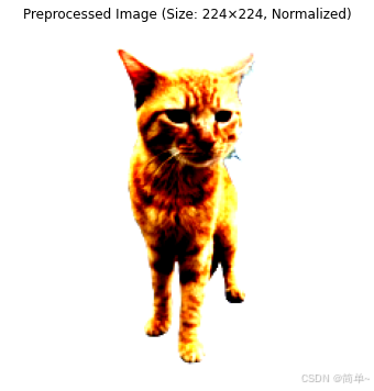
# 显示预处理后的图片
print("\n📸 显示预处理后图片...")
plt.figure(figsize=(8, 6))
plt.imshow(img_numpy)
plt.title("Preprocessed Image (Size: 224×224, Normalized)")  # 图表标题用英文
plt.axis('off')
plt.show()

# ========== 第四部分：加载类别标签信息 ==========

print("\n📂 加载ImageNet类别标签信息...")

# 加载ILSVRC的标签信息文件
# imagenet_class_index.json文件包含1000个类别的信息
# 格式: {"0": ["n01440764", "tench"], "1": ["n01443537", "goldfish"], ...}
try:
    ILSVRC_class_index = json.load(open('./data/imagenet_class_index.json', 'r'))
    print(f"✅ 成功加载类别标签，共 {len(ILSVRC_class_index)} 个类别")
    
    # 显示前几个类别作为示例
    print("\n   前5个类别示例:")
    for i in range(5):
        class_id = str(i)
        wordnet_id, class_name = ILSVRC_class_index[class_id]
        print(f"     {class_id}: {class_name} (WordNet ID: {wordnet_id})")
        
except Exception as e:
    print(f"❌ 无法加载类别标签文件: {e}")
    exit()

# ========== 第五部分：生成预测器实例 ==========

print("\n🤖 创建预测器实例...")
predictor = ILSVRCPredictor(ILSVRC_class_index)
print("✅ 预测器创建成功")

# ========== 第六部分：使用VGG-16进行图片分类 ==========

print("\n🔍 使用VGG-16进行图片分类...")
print("=" * 50)

# 1. 重新读取输入图片（确保原始图片）
try:
    image_file_path = './data/1.jpg'
    img = Image.open(image_file_path)  # 原始PIL图片对象
    print(f"✅ 重新读取图片: {image_file_path}")
except Exception as e:
    print(f"❌ 无法读取图片: {e}")
    exit()

# 2. 应用预处理
print("\n🔧 应用预处理...")
transform = BaseTransform(resize, mean, std)  # 创建预处理类实例
img_transformed = transform(img)  # 返回形状: torch.Size([3, 224, 224])

print(f"   预处理后张量形状: {img_transformed.shape}")

# 3. 添加批次维度
# 神经网络通常需要批次维度: [批次大小, 通道数, 高度, 宽度]
# unsqueeze_(0): 在0维度添加一个维度，从[3,224,224]变为[1,3,224,224]
# 下划线版本表示原地操作（in-place operation）
# 生成VGG-16模型的实例
# use_pretrained = True 表示使用在ImageNet数据集上预训练的权重参数
# 第一次运行时会从网络下载约500MB的模型权重文件
# 在大多数情况下，下载的模型权重文件保存在以下目录中：
# Linux/Unix: ~/.cache/torch/hub/checkpoints/
# Windows: C:\\Users\\<用户名>\\.cache\\torch\\hub\\checkpoints\\
# macOS: ~/.cache/torch/hub/checkpoints/
inputs = img_transformed.unsqueeze_(0)  # torch.Size([1, 3, 224, 224])
print(f"   添加批次维度后形状: {inputs.shape}")

# 4. 验证模型是否已加载
try:
    # 检查net变量是否存在（应该在之前的代码中已定义）
    if 'net' not in locals() and 'net' not in globals():
        print("\n⚠️ 警告: VGG-16模型未加载，正在自动加载...")
        use_pretrained = True
        net = models.vgg16(pretrained=use_pretrained)
        net.eval()  # 设置为评估模式
        print("✅ VGG-16模型加载成功")
    else:
        print("✅ 使用已加载的VGG-16模型")
except Exception as e:
    print(f"❌ 模型加载失败: {e}")
    exit()

# 5. 前向传播（模型推理）
print("\n🧠 运行模型推理...")

# 使用torch.no_grad()上下文管理器
# 作用: 不计算梯度，节省内存，提高推理速度
with torch.no_grad():
    out = net(inputs)  # 输入: torch.Size([1, 3, 224, 224]), 输出: torch.Size([1, 1000])

print(f"   模型输出形状: {out.shape}")
print(f"   输出数据类型: {out.dtype}")

# 6. 后处理：从模型输出获取预测结果
print("\n📊 解析预测结果...")
result = predictor.predict_max(out)

# 7. 输出预测结果
print("\n" + "=" * 50)
print("🎯 预测结果")
print("=" * 50)
print(f"输入图片: {image_file_path}")
print(f"预测类别: {result}")

# 8. 显示前5个最可能的类别
print("\n📈 前5个最可能的类别:")
with torch.no_grad():
    # 获取所有类别的概率（softmax）
    probabilities = torch.nn.functional.softmax(out, dim=1)
    probs_numpy = probabilities.numpy()[0]  # 去除批次维度
    
    # 获取概率最高的5个索引
    top5_indices = np.argsort(probs_numpy)[-5:][::-1]  # 从高到低
    
    for i, idx in enumerate(top5_indices, 1):
        class_name = ILSVRC_class_index[str(idx)][1]
        probability = probs_numpy[idx] * 100
        print(f"  {i}. {class_name}: {probability:.2f}%")

# ========== 第七部分：完整流程总结 ==========

print("\n" + "=" * 60)
print("📋 完整流程总结")
print("=" * 60)

print("""
✅ 流程已完成，步骤总结:

1. 📁 数据准备
   - 读取图片文件 (./data/1.jpg)
   - 转换为PIL.Image对象

2. 🔧 图片预处理
   - 调整尺寸: 224×224
   - 中心裁剪: 确保正方形
   - 张量转换: PIL → torch.Tensor
   - 颜色归一化: 使用ImageNet统计量

3. 🧠 模型推理
   - 添加批次维度: [1, 3, 224, 224]
   - 前向传播: 通过VGG-16网络
   - 获取输出: 1000个类别的概率分布

4. 📊 结果解析
   - 找到最高概率类别
   - 映射到类别名称
   - 显示前5个预测结果

5. 🎯 输出结果
   - 显示预测类别
   - 显示置信度
""")

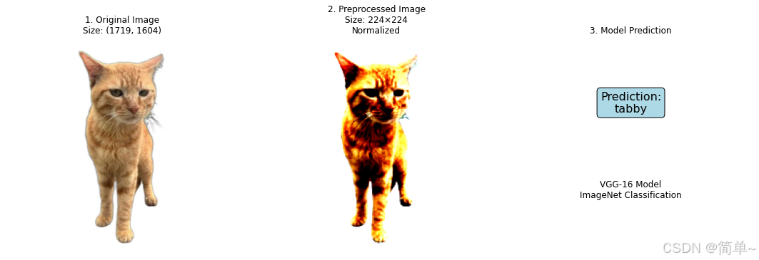
# ========== 第八部分：显示完整对比图 ==========

print("\n📊 生成完整处理流程对比图...")

# 创建子图显示完整流程
fig, axes = plt.subplots(1, 3, figsize=(15, 5))

# 子图1: 原始图片
axes[0].imshow(img)
axes[0].set_title("1. Original Image\n" + f"Size: {img.size}")  # 图表标题用英文
axes[0].axis('off')

# 子图2: 预处理后图片
axes[1].imshow(img_numpy)
axes[1].set_title("2. Preprocessed Image\n" + f"Size: 224×224\nNormalized")  # 图表标题用英文
axes[1].axis('off')

# 子图3: 添加预测结果文本
axes[2].text(0.5, 0.7, f"Prediction:\n{result}",  # 图表文本用英文
            ha='center', va='center', fontsize=16, 
            bbox=dict(boxstyle="round,pad=0.3", facecolor="lightblue"))
axes[2].text(0.5, 0.3, "VGG-16 Model\nImageNet Classification",  # 图表文本用英文
            ha='center', va='center', fontsize=12)
axes[2].set_title("3. Model Prediction")  # 图表标题用英文
axes[2].axis('off')

plt.tight_layout()
plt.show()

print("✅ 完整流程可视化完成！")
print("\n" + "=" * 60)
print("🎉 图片分类流程成功完成！")
print("=" * 60)

5.3处理流程

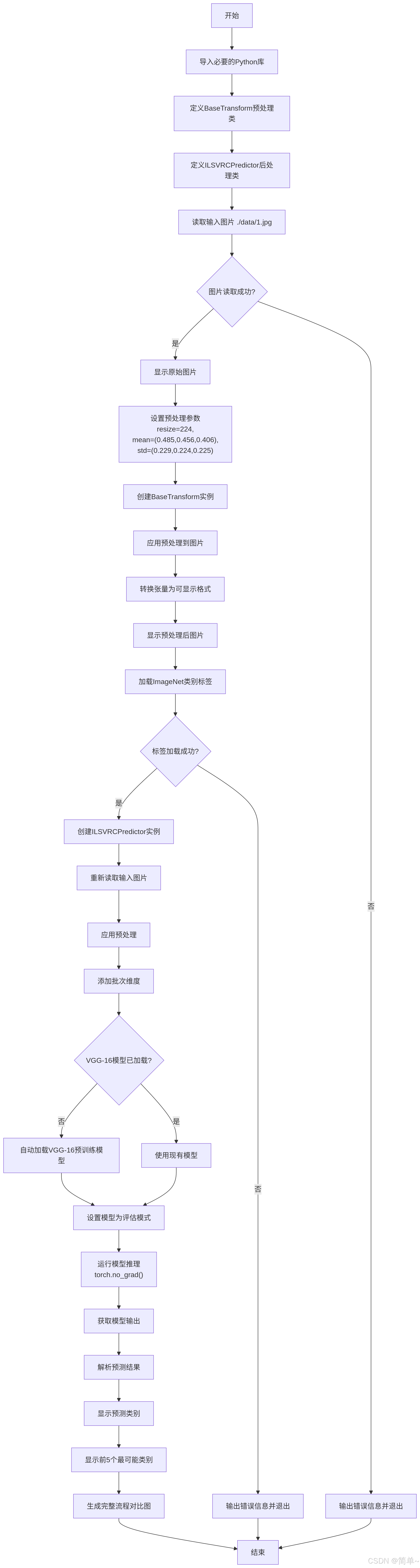
5.4预测结果

🚀 开始验证图片预处理效果...
==================================================
✅ 成功读取图片: ./data/1.jpg
   原始图片尺寸: (1719, 1604) (宽度×高度)
   图片模式: RGB (RGB或L等)

📸 显示原始图片...

🔧 应用预处理转换...
   目标尺寸: 224x224
   均值 (R, G, B): (0.485, 0.456, 0.406)
   标准差 (R, G, B): (0.229, 0.224, 0.225)
   预处理后张量形状: torch.Size([3, 224, 224])
   数据类型: torch.float32
   取值范围: [-1.773, 2.640]

📸 显示预处理后图片...

📂 加载ImageNet类别标签信息...
✅ 成功加载类别标签，共 1000 个类别

   前5个类别示例:
     0: tench (WordNet ID: n01440764)
     1: goldfish (WordNet ID: n01443537)
     2: great_white_shark (WordNet ID: n01484850)
     3: tiger_shark (WordNet ID: n01491361)
     4: hammerhead (WordNet ID: n01494475)

🤖 创建预测器实例...
✅ 预测器创建成功

🔍 使用VGG-16进行图片分类...
==================================================
✅ 重新读取图片: ./data/1.jpg

🔧 应用预处理...
   预处理后张量形状: torch.Size([3, 224, 224])
   添加批次维度后形状: torch.Size([1, 3, 224, 224])
✅ 使用已加载的VGG-16模型

🧠 运行模型推理...
   模型输出形状: torch.Size([1, 1000])
   输出数据类型: torch.float32

📊 解析预测结果...

==================================================
🎯 预测结果
==================================================
输入图片: ./data/1.jpg
预测类别: tabby

📈 前5个最可能的类别:
  1. tabby: 42.64%
  2. Egyptian_cat: 33.12%
  3. tiger_cat: 20.21%
  4. lynx: 0.77%
  5. bow_tie: 0.14%

============================================================
📋 完整流程总结
============================================================

✅ 流程已完成，步骤总结:

1. 📁 数据准备
   - 读取图片文件 (./data/1.jpg)
   - 转换为PIL.Image对象

2. 🔧 图片预处理
   - 调整尺寸: 224×224
   - 中心裁剪: 确保正方形
   - 张量转换: PIL → torch.Tensor
   - 颜色归一化: 使用ImageNet统计量

3. 🧠 模型推理
   - 添加批次维度: [1, 3, 224, 224]
   - 前向传播: 通过VGG-16网络
   - 获取输出: 1000个类别的概率分布

4. 📊 结果解析
   - 找到最高概率类别
   - 映射到类别名称
   - 显示前5个预测结果

5. 🎯 输出结果
   - 显示预测类别
   - 显示置信度

📊 生成完整处理流程对比图...

✅ 完整流程可视化完成！

============================================================
🎉 图片分类流程成功完成！
============================================================

tabby，橘座本座

六、性能优化技巧

6.1 内存优化

# 1. 使用梯度检查点
from torch.utils.checkpoint import checkpoint

class MemoryEfficientVGG(nn.Module):
    def forward(self, x):
        # 使用检查点减少内存占用
        x = checkpoint(self.features1, x)
        x = checkpoint(self.features2, x)
        x = checkpoint(self.features3, x)
        x = checkpoint(self.features4, x)
        x = checkpoint(self.features5, x)
        return x

# 2. 使用混合精度训练
from torch.cuda.amp import autocast, GradScaler

scaler = GradScaler()
with autocast():
    output = model(input)
    loss = criterion(output, target)
scaler.scale(loss).backward()
scaler.step(optimizer)
scaler.update()

6.2 推理加速

# 1. 模型量化
quantized_model = torch.quantization.quantize_dynamic(
    model, {nn.Linear}, dtype=torch.qint8
)

# 2. TorchScript优化
scripted_model = torch.jit.script(model)
scripted_model.save('vgg16_scripted.pt')

# 3. ONNX导出
torch.onnx.export(
    model, 
    dummy_input, 
    "vgg16.onnx",
    input_names=['input'],
    output_names=['output'],
    dynamic_axes={'input': {0: 'batch_size'}}
)

七、VGG-16的现代替代方案

模型	提出年份	核心创新	参数量	ImageNet Top-1准确率
VGG-16	2014	小卷积核堆叠	1.38亿	71.3%
ResNet-50	2015	残差连接	2560万	76.2%
Inception-v3	2015	多尺度卷积	2380万	78.8%
EfficientNet-B0	2019	复合缩放	530万	77.1%
Vision Transformer	2020	自注意力机制	8600万	77.9%