如果以面向对象(OOP)的方式进行BP神经网络系统的设计与实践的话，因为权值的初始化以及类的构造都只进行一次（而且发生在整个流程的开始阶段），所以自然地将权值（全部层layer之间的全部权值）初始化的过程放在类的构函数中，而权值的初始化，一种trivial常用的初始化方法为，对各个权值使用均值为0方差为1的正态分布（也即np.random.randn(shape)）进行初始化，也即：

class Network(object):
    # topology：表示神经网络拓扑结构，用list或者tuple来实现，
    # 比如[784, 30, 10]，表示784个神经元的输入层，30个neuron的隐层，以及十个neuron的输出层
    def __init__(self, topology):
        self.topology = topology
        self.num_layers = len(topology)
        self.biases = [np.random.randn(y, 1) for y in topology[1:]]
        self.weights = [np.random.randn(y, x) for x, y in zip(self.weights[:-1], self.weights[1:])]

我们不妨以一个简单的具体例子，分析这种初始化方法可能存在的缺陷，如下图所示：

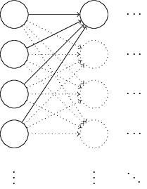
为了简化问题，我们只以最左一层向中间一层的第一个神经元（neuron）进行前向（forward）传递为例进行分析，假设一个输入样本（特征向量，x<script type="math/tex" id="MathJax-Element-1059">x</script>，维度为1000），一半为1，一半为0（这样的假设很特殊，但也很能说明问题），根据前向传递公式，z=∑jwjxj+b<script type="math/tex" id="MathJax-Element-1060">z=\sum_jw_jx_j+b</script>，z<script type="math/tex" id="MathJax-Element-1061">z</script>即为输入层向中间隐层第一个神经元的输入。因为输入的一半为0的缘故，再根据前文以及代码也即权重和偏置初始化为独立同分布的标准高斯随机变量，z<script type="math/tex" id="MathJax-Element-1062">z</script>为501（500个权值+1个偏置）个标准正太随机变量的和，由独立随机变量和的方差等于方差的和可知，因此z<script type="math/tex" id="MathJax-Element-1063">z</script>的分布服从0均值，标准差为501−−−√≈22.4<script type="math/tex" id="MathJax-Element-1064">\sqrt{501}\approx 22.4</script>，标准差从1升高到22.4，由高斯密度函数f(x)=12π√σexp(−(x−μ)2σ2)<script type="math/tex" id="MathJax-Element-1065">f(x)=\frac1{\sqrt{2\pi}\sigma}\exp(\frac{-(x-\mu)^2}{\sigma^2})</script>可知，方差越大，密度函数的分布越扁平，也即分布越均匀而不是集中在一段区域，其概率密度函数为（可见十分平坦）：

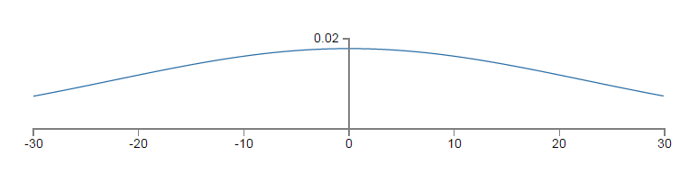
以上的平坦的概率密度函数为z<script type="math/tex" id="MathJax-Element-1066">z</script>的pdf（概率密度函数），因为pdf较为均匀，|z|<script type="math/tex" id="MathJax-Element-1067">|z|</script>的值就不会像N∼(0,1)<script type="math/tex" id="MathJax-Element-1068">\mathcal{N}\sim(0,1)</script>那样集中于均值附近（越远离均值中心，密度值会迅速衰减），而会以更大的概率取更大的值。这中初始化机制可能带来什么样的问题呢？|z|<script type="math/tex" id="MathJax-Element-1069">|z|</script>取值很大，也即z≫1<script type="math/tex" id="MathJax-Element-1070">z\gg 1</script>或者z≪−1<script type="math/tex" id="MathJax-Element-1071">z\ll -1</script>，相应的该神经元的activation值σ(z)<script type="math/tex" id="MathJax-Element-1072">\sigma(z)</script>就会接近0或者1，而我们知道，如下图示，σ(z)<script type="math/tex" id="MathJax-Element-1073">\sigma(z)</script>越靠近0或者1其变化率越小，也即是达到一种饱和（saturate）状态。

而权值更新公式为：

<script type="math/tex; mode=display" id="MathJax-Element-1074">\frac{\partial\,C}{\partial\,w^L}=(a^L-y)\sigma'(z)</script>
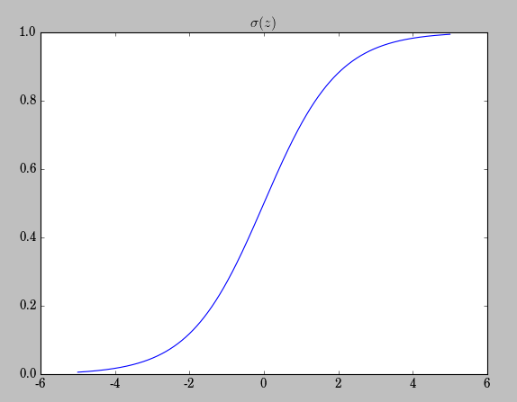
也就意味着越小的σ′(z)<script type="math/tex" id="MathJax-Element-1075">\sigma'(z)</script>，越小的梯度更新，同等学习率（learning rate：η<script type="math/tex" id="MathJax-Element-1076">\eta</script>）的情况下，越小的学习速率。

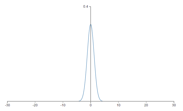
如何进行改进呢？假使输入层有nin<script type="math/tex" id="MathJax-Element-1077">n_{in}</script>个神经元，我们可将这些神经元对应的权重初始化为0均值，标准差为1/(√nin)<script type="math/tex" id="MathJax-Element-1078">1/\sqrt(n_{in})</script>，这样，高斯pdf的形式将会趋于陡峭，而不是上文的平坦，σ′(z)<script type="math/tex" id="MathJax-Element-1079">\sigma'(z)</script>将以较小的概率达到饱和状态。仍以上文的设置为基础，我们来分析，现在z<script type="math/tex" id="MathJax-Element-1080">z</script>的pdf，均值为0，标准差为500/1000−−−−−−−−√≈0.707<script type="math/tex" id="MathJax-Element-1081">\sqrt{500/1000}\approx 0.707</script>，其形式如下：

相关代码：

def default_weight_init(self):
    self.biases = [np.random.randn(y, 1)/y for y in self.topology[1:]] 
    self.weights = [np.random.rand(y, x)/np.sqrt(x) for x, y in zip(self.topology[:-1], self.topology[1:])]

def large_weight_init(self):
    self.biases = [np.random.randn(y, 1) for y in self.topoloy[1:]]
    self.weights = [np.random.randn(y, x)/np.sqrt(x) for x, y in zip(self.topology[:-1], self.topology[1:])]

我们看到正是这样一种np.random.randn(y, x)向np.random.randn(y, x)/np.sqrt(x)小小的改变，却暗含着丰富的概率论与数理统计的知识，可见无时无刻无处不体现着数学工具的强大。