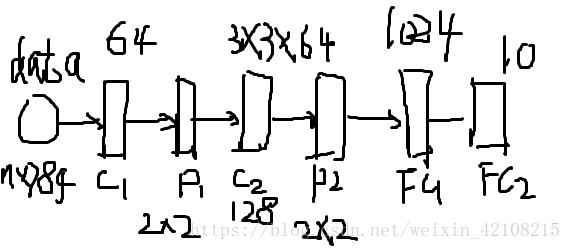
继昨天夜里构建的三层神经网络的惨淡的精确度，接下来构建卷积神经网络去干这个10分类的任务，效果会怎么样呢？还是很棒的,下面画一个草图来表示网络结构：

import numpy as np
import tensorflow as tf
import matplotlib.pyplot as plt
import input_data
mnist = input_data.read_data_sets('data/', one_hot=True)
trainimg   = mnist.train.images
trainlabel = mnist.train.labels
testimg    = mnist.test.images
testlabel  = mnist.test.labels
print ("MNIST ready")
n_input  = 784
n_output = 10
weights  = {
        'wc1': tf.Variable(tf.random_normal([3, 3, 1, 64], stddev=0.1)),#【h,w,d,out】由于是灰度图只有有个通道所以深度是1
        'wc2': tf.Variable(tf.random_normal([3, 3, 64, 128], stddev=0.1)),
        'wd1': tf.Variable(tf.random_normal([7*7*128, 1024], stddev=0.1)),#这个7*7是两层卷积和池化后输出到全连接层的连接，直接套公式计算
        'wd2': tf.Variable(tf.random_normal([1024, n_output], stddev=0.1))
    }
biases   = {
        'bc1': tf.Variable(tf.random_normal([64], stddev=0.1)),#这个是bias偏移项，其大小跟着所在层的输出
        'bc2': tf.Variable(tf.random_normal([128], stddev=0.1)),
        'bd1': tf.Variable(tf.random_normal([1024], stddev=0.1)),
        'bd2': tf.Variable(tf.random_normal([n_output], stddev=0.1))
    }
def conv_basic(_input, _w, _b, _keepratio):
        # INPUT
        _input_r = tf.reshape(_input, shape=[-1, 28, 28, 1])#【n,h,w,d】大小 长 宽 深度
        # CONV LAYER 1
        _conv1 = tf.nn.conv2d(_input_r, _w['wc1'], strides=[1, 1, 1, 1], padding='SAME')#这个strides用过caffe我们知道直接在文档里设置就好，那么这里为什么用四个数呢，这个是tensorflow的格式
        #_mean, _var = tf.nn.moments(_conv1, [0, 1, 2])
        #_conv1 = tf.nn.batch_normalization(_conv1, _mean, _var, 0, 1, 0.0001)
        _conv1 = tf.nn.relu(tf.nn.bias_add(_conv1, _b['bc1']))#我们可以在卷积之后加个relu函数，加强非线性
        _pool1 = tf.nn.max_pool(_conv1, ksize=[1, 2, 2, 1], strides=[1, 2, 2, 1], padding='SAME')#这个padding设置为same就是在滑动窗口移动，数字不够时补0用的
        _pool_dr1 = tf.nn.dropout(_pool1, _keepratio)#这个是我们用于正则化的，我们让他过去多少就过去多少，比如设置成0.5，那就只有一半能够通过
        # CONV LAYER 2
        _conv2 = tf.nn.conv2d(_pool_dr1, _w['wc2'], strides=[1, 1, 1, 1], padding='SAME')
        #_mean, _var = tf.nn.moments(_conv2, [0, 1, 2])
        #_conv2 = tf.nn.batch_normalization(_conv2, _mean, _var, 0, 1, 0.0001)
        _conv2 = tf.nn.relu(tf.nn.bias_add(_conv2, _b['bc2']))
        _pool2 = tf.nn.max_pool(_conv2, ksize=[1, 2, 2, 1], strides=[1, 2, 2, 1], padding='SAME')
        _pool_dr2 = tf.nn.dropout(_pool2, _keepratio)
        # VECTORIZE
        _dense1 = tf.reshape(_pool_dr2, [-1, _w['wd1'].get_shape().as_list()[0]])#这个全连接层有个窍门，通过这句代码转换成tensorflow所要的格式，然后直接输出这个大小
        # FULLY CONNECTED LAYER 1
        _fc1 = tf.nn.relu(tf.add(tf.matmul(_dense1, _w['wd1']), _b['bd1']))
        _fc_dr1 = tf.nn.dropout(_fc1, _keepratio)
        # FULLY CONNECTED LAYER 2
        _out = tf.add(tf.matmul(_fc_dr1, _w['wd2']), _b['bd2'])
        # RETURN
        out = { 'input_r': _input_r, 'conv1': _conv1, 'pool1': _pool1, 'pool1_dr1': _pool_dr1,
            'conv2': _conv2, 'pool2': _pool2, 'pool_dr2': _pool_dr2, 'dense1': _dense1,
            'fc1': _fc1, 'fc_dr1': _fc_dr1, 'out': _out
        }
        return out
print ("CNN READY")

a = tf.Variable(tf.random_normal([3, 3, 1, 64], stddev=0.1))
print (a)
a = tf.Print(a, [a], "a: ")
init = tf.global_variables_initializer()
sess = tf.Session()
sess.run(init)
#sess.run(a)
x = tf.placeholder(tf.float32, [None, n_input])
y = tf.placeholder(tf.float32, [None, n_output])
keepratio = tf.placeholder(tf.float32)

# FUNCTIONS

_pred = conv_basic(x, weights, biases, keepratio)['out']
cost = tf.reduce_mean(tf.nn.softmax_cross_entropy_with_logits(logits=_pred, labels=y))
optm = tf.train.AdamOptimizer(learning_rate=0.001).minimize(cost)
_corr = tf.equal(tf.argmax(_pred,1), tf.argmax(y,1)) 
accr = tf.reduce_mean(tf.cast(_corr, tf.float32)) 
init = tf.global_variables_initializer()
    
# SAVER
print ("GRAPH READY")
sess = tf.Session()
sess.run(init)

training_epochs = 15
batch_size      = 16
display_step    = 1
for epoch in range(training_epochs):
    avg_cost = 0.
    #total_batch = int(mnist.train.num_examples/batch_size)
    total_batch = 10
    # Loop over all batches
    for i in range(total_batch):
        batch_xs, batch_ys = mnist.train.next_batch(batch_size)
        # Fit training using batch data
        sess.run(optm, feed_dict={x: batch_xs, y: batch_ys, keepratio:0.7})
        # Compute average loss
        avg_cost += sess.run(cost, feed_dict={x: batch_xs, y: batch_ys, keepratio:1.})/total_batch

    # Display logs per epoch step
    if epoch % display_step == 0: 
        print ("Epoch: %03d/%03d cost: %.9f" % (epoch, training_epochs, avg_cost))
        train_acc = sess.run(accr, feed_dict={x: batch_xs, y: batch_ys, keepratio:1.})
        print (" Training accuracy: %.3f" % (train_acc))
        #test_acc = sess.run(accr, feed_dict={x: testimg, y: testlabel, keepratio:1.})
        #print (" Test accuracy: %.3f" % (test_acc))

print ("OPTIMIZATION FINISHED")
打印结果如下：
Epoch: 000/015 cost: 4.536491299
 Training accuracy: 0.438
Epoch: 001/015 cost: 2.044470596
 Training accuracy: 0.688
Epoch: 002/015 cost: 1.237399143
 Training accuracy: 0.625
Epoch: 003/015 cost: 1.235728055
 Training accuracy: 0.688
Epoch: 004/015 cost: 1.185478628
 Training accuracy: 0.625
Epoch: 005/015 cost: 1.095422560
 Training accuracy: 0.750
Epoch: 006/015 cost: 1.009366870
 Training accuracy: 1.000
Epoch: 007/015 cost: 0.885777467
 Training accuracy: 1.000
Epoch: 008/015 cost: 0.770399562
 Training accuracy: 0.812
Epoch: 009/015 cost: 0.617595312
 Training accuracy: 0.938
Epoch: 010/015 cost: 0.562738934
 Training accuracy: 1.000
Epoch: 011/015 cost: 0.585591027
 Training accuracy: 0.750
Epoch: 012/015 cost: 0.412116882
 Training accuracy: 0.938
Epoch: 013/015 cost: 0.422649217
 Training accuracy: 0.938
Epoch: 014/015 cost: 0.417875010
 Training accuracy: 0.938
OPTIMIZATION FINISHED

从逻辑回归到二层神经网络，到三层神经网络，紧接着到这个卷积神经网对比这个精确度，我们可以看到卷积神经网络还是蛮强大的，把昨天那个惨淡的精确度的阴影给磨掉了，再接再厉