点击上方“Python爬虫与数据挖掘”，进行关注

回复“书籍”即可获赠Python从入门到进阶共10本电子书

今

日

鸡

汤

苟利国家生死以，岂因祸福避趋之。——林则徐《赴戍登程口占示家人》

---

作者：Python进阶者

关键词：机器学习, 数据预处理, 特征工程, 模型训练, 超参数优化, 模型部署, Scikit-learn, TensorFlow

开头引言：

机器学习已成为数据驱动决策的核心技术。本文通过一个完整的案例，展示如何使用Python完成从数据准备到模型部署的全流程，帮助你快速掌握机器学习实战技能。

一、数据准备与探索

1.1 数据加载与质量检查

import pandas as pd
import numpy as np
import matplotlib.pyplot as plt
import seaborn as sns
from sklearn.datasets import load_iris

# 加载示例数据
defload_and_explore_data():
"""数据加载与探索"""
# 使用鸢尾花数据集示例
    iris = load_iris()
    df = pd.DataFrame(iris.data, columns=iris.feature_names)
    df['target'] = iris.target
    df['species'] = df['target'].map({0: 'setosa', 1: 'versicolor', 2: 'virginica'})

print("=== 数据概览 ===")
print(f"数据形状: {df.shape}")
print("\n前5行数据:")
print(df.head())

print("\n基本统计信息:")
print(df.describe())

print("\n缺失值检查:")
print(df.isnull().sum())

return df

# 数据可视化
defvisualize_data(df):
"""数据可视化分析"""
    fig, axes = plt.subplots(2, 2, figsize=(12, 10))

# 特征分布
    df[iris.feature_names].hist(ax=axes[0, 0])
    axes[0, 0].set_title('特征分布')

# 类别分布
    df['species'].value_counts().plot(kind='bar', ax=axes[0, 1])
    axes[0, 1].set_title('类别分布')

# 散点图
    sns.scatterplot(data=df, x='sepal length (cm)', y='sepal width (cm)', 
                   hue='species', ax=axes[1, 0])
    axes[1, 0].set_title('花萼长度 vs 花萼宽度')

# 相关性热图
    numeric_df = df.select_dtypes(include=[np.number])
    sns.heatmap(numeric_df.corr(), annot=True, ax=axes[1, 1])
    axes[1, 1].set_title('相关性热图')

    plt.tight_layout()
    plt.show()

# 执行数据探索
df = load_and_explore_data()
visualize_data(df)

1.2 数据预处理

from sklearn.preprocessing import StandardScaler, LabelEncoder
from sklearn.model_selection import train_test_split

defpreprocess_data(df):
"""数据预处理流程"""
print("=== 数据预处理 ===")

# 复制数据避免修改原数据
    data = df.copy()

# 处理缺失值（示例数据无缺失，展示流程）
if data.isnull().sum().sum() > 0:
# 数值型用中位数填充
        numeric_cols = data.select_dtypes(include=[np.number]).columns
        data[numeric_cols] = data[numeric_cols].fillna(data[numeric_cols].median())

# 类别型用众数填充
        categorical_cols = data.select_dtypes(include=['object']).columns
for col in categorical_cols:
            data[col] = data[col].fillna(data[col].mode()[0] ifnot data[col].mode().empty else'Unknown')

# 特征工程：创建新特征
    data['sepal_ratio'] = data['sepal length (cm)'] / data['sepal width (cm)']
    data['petal_ratio'] = data['petal length (cm)'] / data['petal width (cm)']

print("创建的新特征:")
print(data[['sepal_ratio', 'petal_ratio']].describe())

return data

defprepare_features_target(data, target_col='species'):
"""准备特征和目标变量"""
# 选择特征
    feature_cols = [col for col in data.columns if col notin [target_col, 'target']]
    X = data[feature_cols]
    y = data[target_col]

# 编码目标变量（如果是字符串标签）
if y.dtype == 'object':
        le = LabelEncoder()
        y_encoded = le.fit_transform(y)
else:
        y_encoded = y

# 数据标准化
    scaler = StandardScaler()
    X_scaled = scaler.fit_transform(X)

# 划分训练测试集
    X_train, X_test, y_train, y_test = train_test_split(
        X_scaled, y_encoded, test_size=0.2, random_state=42, stratify=y_encoded
    )

print(f"训练集: {X_train.shape}, 测试集: {X_test.shape}")
return X_train, X_test, y_train, y_test, scaler, feature_cols

# 执行预处理
processed_data = preprocess_data(df)
X_train, X_test, y_train, y_test, scaler, feature_names = prepare_features_target(processed_data)

二、模型训练与评估

2.1 多种算法比较

from sklearn.linear_model import LogisticRegression
from sklearn.ensemble import RandomForestClassifier
from sklearn.svm import SVC
from sklearn.neighbors import KNeighborsClassifier
from sklearn.metrics import classification_report, confusion_matrix, accuracy_score

deftrain_and_evaluate_models(X_train, X_test, y_train, y_test):
"""训练并评估多个模型"""
print("=== 模型训练与评估 ===")

# 定义模型
    models = {
'逻辑回归': LogisticRegression(random_state=42, max_iter=1000),
'随机森林': RandomForestClassifier(random_state=42, n_estimators=100),
'支持向量机': SVC(random_state=42, probability=True),
'K近邻': KNeighborsClassifier(n_neighbors=3)
    }

    results = {}

for name, model in models.items():
print(f"\n训练 {name}...")

# 训练模型
        model.fit(X_train, y_train)

# 预测
        y_pred = model.predict(X_test)
        y_pred_proba = model.predict_proba(X_test)

# 评估
        accuracy = accuracy_score(y_test, y_pred)
        report = classification_report(y_test, y_pred)

        results[name] = {
'model': model,
'accuracy': accuracy,
'predictions': y_pred,
'probabilities': y_pred_proba,
'report': report
        }

print(f"{name} 准确率: {accuracy:.4f}")

return results

defcompare_models(results):
"""比较模型性能"""
print("\n=== 模型比较 ===")

# 准确率比较
    accuracies = {name: result['accuracy'] for name, result in results.items()}
    best_model = max(accuracies, key=accuracies.get)

print("各模型准确率:")
for name, accuracy insorted(accuracies.items(), key=lambda x: x[1], reverse=True):
print(f"  {name}: {accuracy:.4f}")

print(f"\n最佳模型: {best_model} (准确率: {accuracies[best_model]:.4f})")

# 可视化比较
    plt.figure(figsize=(10, 6))
    models = list(accuracies.keys())
    scores = list(accuracies.values())

    bars = plt.bar(models, scores, color=['skyblue', 'lightcoral', 'lightgreen', 'gold'])
    plt.title('模型准确率比较')
    plt.ylabel('准确率')
    plt.ylim(0, 1.0)

# 在柱子上添加数值
for bar, score inzip(bars, scores):
        plt.text(bar.get_x() + bar.get_width()/2, bar.get_height() + 0.01,
f'{score:.4f}', ha='center', va='bottom')

    plt.xticks(rotation=45)
    plt.tight_layout()
    plt.show()

return best_model

# 训练和评估模型
model_results = train_and_evaluate_models(X_train, X_test, y_train, y_test)
best_model_name = compare_models(model_results)
best_model = model_results[best_model_name]['model']

2.2 模型优化

from sklearn.model_selection import GridSearchCV

defoptimize_model(X_train, y_train):
"""超参数优化"""
print("=== 超参数优化 ===")

# 使用随机森林进行优化示例
    param_grid = {
'n_estimators': [50, 100, 200],
'max_depth': [3, 5, 7, None],
'min_samples_split': [2, 5, 10],
'min_samples_leaf': [1, 2, 4]
    }

    rf = RandomForestClassifier(random_state=42)
    grid_search = GridSearchCV(
        rf, param_grid, cv=5, scoring='accuracy', n_jobs=-1, verbose=1
    )

    grid_search.fit(X_train, y_train)

print(f"最佳参数: {grid_search.best_params_}")
print(f"最佳交叉验证分数: {grid_search.best_score_:.4f}")

return grid_search.best_estimator_

# 模型优化
optimized_model = optimize_model(X_train, y_train)

# 评估优化后的模型
optimized_accuracy = accuracy_score(y_test, optimized_model.predict(X_test))
print(f"优化后模型测试准确率: {optimized_accuracy:.4f}")

# 特征重要性分析
ifhasattr(optimized_model, 'feature_importances_'):
    feature_importance = pd.DataFrame({
'feature': feature_names,
'importance': optimized_model.feature_importances_
    }).sort_values('importance', ascending=False)

print("\n特征重要性:")
print(feature_importance)

# 可视化特征重要性
    plt.figure(figsize=(10, 6))
    plt.barh(feature_importance['feature'], feature_importance['importance'])
    plt.title('特征重要性')
    plt.xlabel('重要性')
    plt.tight_layout()
    plt.show()

三、模型部署与应用

3.1 模型保存与加载

import joblib
import json
from datetime import datetime

defsave_model(model, scaler, feature_names, model_name='iris_classifier'):
"""保存模型和相关组件"""
print("=== 保存模型 ===")

# 创建时间戳
    timestamp = datetime.now().strftime("%Y%m%d_%H%M%S")

# 保存模型
    model_filename = f'{model_name}_{timestamp}.joblib'
    joblib.dump(model, model_filename)

# 保存预处理对象
    preprocessing_filename = f'{model_name}_preprocessing_{timestamp}.joblib'
    preprocessing_artifacts = {
'scaler': scaler,
'feature_names': feature_names,
'timestamp': timestamp
    }
    joblib.dump(preprocessing_artifacts, preprocessing_filename)

# 保存模型信息
    model_info = {
'model_name': model_name,
'model_type': type(model).__name__,
'features': feature_names,
'timestamp': timestamp,
'version': '1.0.0'
    }

    info_filename = f'{model_name}_info_{timestamp}.json'
withopen(info_filename, 'w') as f:
        json.dump(model_info, f, indent=2)

print(f"模型保存为: {model_filename}")
print(f"预处理对象保存为: {preprocessing_filename}")
print(f"模型信息保存为: {info_filename}")

return {
'model_file': model_filename,
'preprocessing_file': preprocessing_filename,
'info_file': info_filename
    }

defload_model(model_files):
"""加载模型和相关组件"""
print("=== 加载模型 ===")

# 加载模型
    model = joblib.load(model_files['model_file'])

# 加载预处理对象
    preprocessing = joblib.load(model_files['preprocessing_file'])

# 加载模型信息
withopen(model_files['info_file'], 'r') as f:
        model_info = json.load(f)

print(f"加载模型: {model_info['model_name']}")
print(f"模型类型: {model_info['model_type']}")
print(f"特征数量: {len(model_info['features'])}")

return model, preprocessing, model_info

# 保存模型
saved_files = save_model(optimized_model, scaler, feature_names)

# 加载模型（演示用途）
loaded_model, loaded_preprocessing, model_info = load_model(saved_files)

3.2 创建预测API

from flask import Flask, request, jsonify
import numpy as np

defcreate_prediction_api(model, preprocessing):
"""创建预测API"""
classPredictionAPI:
def__init__(self, model, preprocessing):
self.model = model
self.scaler = preprocessing['scaler']
self.feature_names = preprocessing['feature_names']

defpredict(self, features):
"""单个预测"""
# 转换为numpy数组并重塑
            features_array = np.array(features).reshape(1, -1)

# 标准化特征
            features_scaled = self.scaler.transform(features_array)

# 预测
            prediction = self.model.predict(features_scaled)[0]
            probability = self.model.predict_proba(features_scaled)[0]

return {
'prediction': int(prediction),
'probabilities': probability.tolist(),
'class_mapping': {0: 'setosa', 1: 'versicolor', 2: 'virginica'}
            }

defbatch_predict(self, features_list):
"""批量预测"""
            predictions = []
for features in features_list:
try:
                    result = self.predict(features)
                    predictions.append(result)
except Exception as e:
                    predictions.append({'error': str(e)})
return predictions

# 创建API实例
    api = PredictionAPI(model, preprocessing)

# 测试预测
print("=== API测试 ===")
    test_features = [5.1, 3.5, 1.4, 0.2, 13.5, 7.0]  # 示例特征
    result = api.predict(test_features)

print("预测结果:")
print(f"预测类别: {result['class_mapping'][result['prediction']]}")
print(f"各类别概率: {result['probabilities']}")

return api

# 创建预测API
prediction_api = create_prediction_api(loaded_model, loaded_preprocessing)

3.3 简单的Web应用

defcreate_simple_web_app(api):
"""创建简单的Web应用"""
    app = Flask(__name__)

    @app.route('/')
defhome():
return'''
        <h1>鸢尾花分类器</h1>
        <p>使用机器学习模型预测鸢尾花种类</p>
        <p>访问 /predict 进行预测</p>
        '''

    @app.route('/predict', methods=['POST'])
defpredict():
try:
            data = request.get_json()

if'features'notin data:
return jsonify({'error': '缺少features参数'}), 400

            features = data['features']

iflen(features) != len(api.feature_names):
return jsonify({
'error': f'特征数量错误，期望{len(api.feature_names)}个特征',
'expected_features': api.feature_names
                }), 400

            result = api.predict(features)
return jsonify(result)

except Exception as e:
return jsonify({'error': str(e)}), 500

    @app.route('/health', methods=['GET'])
defhealth_check():
return jsonify({'status': 'healthy', 'timestamp': datetime.now().isoformat()})

# 生成使用示例代码（不实际运行服务器）
    usage_example = '''
    # 使用示例:
    # import requests
    # 
    # data = {
    #     "features": [5.1, 3.5, 1.4, 0.2, 13.5, 7.0]
    # }
    # 
    # response = requests.post('http://localhost:5000/predict', json=data)
    # print(response.json())
    '''

print("Web应用代码已生成")
print(usage_example)

return app

# 创建Web应用（演示用途）
web_app = create_simple_web_app(prediction_api)

# 注意：实际运行需要取消注释下面的代码
# if __name__ == '__main__':
#     web_app.run(debug=True, host='0.0.0.0', port=5000)

四、模型监控与维护

4.1 性能监控

defsetup_model_monitoring(model, X_test, y_test):
"""设置模型监控"""
print("=== 模型监控设置 ===")

classModelMonitor:
def__init__(self, model, baseline_accuracy=0.9):
self.model = model
self.baseline_accuracy = baseline_accuracy
self.performance_history = []
self.prediction_count = 0

deflog_prediction(self, features, actual, predicted):
"""记录预测结果"""
self.prediction_count += 1
            is_correct = actual == predicted

# 简单的性能跟踪（实际应用中应更复杂）
ifself.prediction_count % 100 == 0:  # 每100次预测计算一次准确率
                recent_predictions = self.performance_history[-100:] iflen(self.performance_history) >= 100elseself.performance_history
if recent_predictions:
                    current_accuracy = sum(p['correct'] for p in recent_predictions) / len(recent_predictions)

if current_accuracy < self.baseline_accuracy * 0.9:  # 性能下降10%
print(f"警告: 模型性能下降! 当前准确率: {current_accuracy:.4f}")

            prediction_record = {
'timestamp': datetime.now().isoformat(),
'features': features,
'actual': actual,
'predicted': predicted,
'correct': is_correct
            }

self.performance_history.append(prediction_record)
return is_correct

defget_performance_metrics(self, window_size=100):
"""获取性能指标"""
iflen(self.performance_history) == 0:
return {'accuracy': 0, 'total_predictions': 0}

            recent_predictions = self.performance_history[-window_size:]
            accuracy = sum(p['correct'] for p in recent_predictions) / len(recent_predictions)

return {
'accuracy': accuracy,
'total_predictions': len(self.performance_history),
'window_size': len(recent_predictions)
            }

# 创建监控器
    monitor = ModelMonitor(model)

# 模拟一些预测记录
    y_pred = model.predict(X_test)
for i, (actual, predicted) inenumerate(zip(y_test, y_pred)):
        features = X_test[i].tolist()
        monitor.log_prediction(features, actual, predicted)

if i >= 50:  # 只模拟50次
break

# 检查性能
    metrics = monitor.get_performance_metrics()
print(f"当前准确率: {metrics['accuracy']:.4f}")
print(f"总预测次数: {metrics['total_predictions']}")

return monitor

# 设置监控
model_monitor = setup_model_monitoring(optimized_model, X_test, y_test)

总结

本文通过一个完整的机器学习项目，展示了从数据准备到模型部署的全流程：

关键步骤回顾：

1. 数据探索与预处理

• 数据质量检查与可视化

• 特征工程与标准化

• 训练测试集划分

• 模型训练与优化

• • 多种算法比较

  • 超参数调优

  • 特征重要性分析

• 模型部署

• • 模型保存与加载

  • API服务创建

  • Web应用开发

• 监控维护

• • 性能监控设置

  • 预测结果跟踪

  实践建议：

  • 🎯 从小开始：从简单数据集开始，逐步复杂化

  • 📊 重视数据质量：数据质量决定模型上限

  • 🔄 持续迭代：机器学习是持续改进的过程

  • 📝 文档化：记录每个步骤和决策

  扩展学习：

  想要进一步深入学习，可以探索：

  • 深度学习模型（神经网络）

  • 自动化机器学习（AutoML）

  • 大数据处理（Spark MLlib）

  • 云平台部署（AWS SageMaker, Azure ML）

  ---

  

  互动话题：你在机器学习项目中遇到过哪些挑战？最想了解哪个环节的深入内容？欢迎在评论区分享你的经验！

  下一篇预告：《Python数据分析实战：Pandas与NumPy高效数据处理》将深入探索数据清洗、转换、聚合等高级技巧，帮助你成为数据处理专家。

  【创作声明】

  本文的核心大纲和部分基础内容由AI辅助生成，但包含了大量笔者的个人实践经验、独家案例和深度解读。所有配图均为笔者定制化AI生成/制作。旨在为大家提供最直观易懂的教程。感谢AI工具提升了我的创作效率。转载请注明出处。欢迎分享和关注，获取更多Python技术干货！

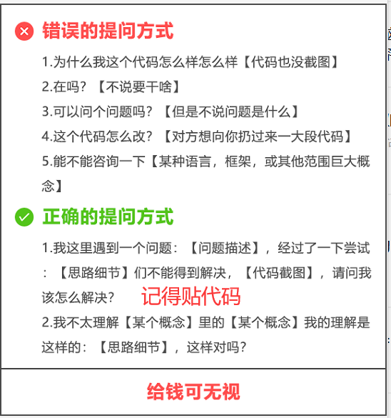
  【提问补充】温馨提示，大家在群里提问的时候。可以注意下面几点：如果涉及到大文件数据，可以数据脱敏后，发点demo数据来（小文件的意思），然后贴点代码（可以复制的那种），记得发报错截图（截全）。代码不多的话，直接发代码文字即可，代码超过50行这样的话，发个.py文件就行。

  

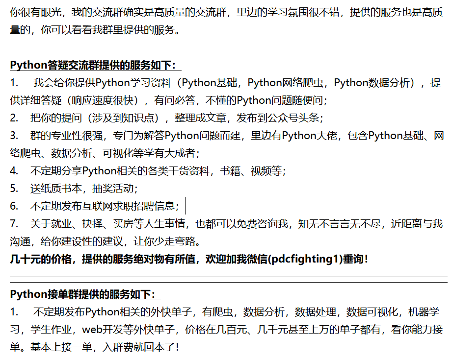
  大家在学习过程中如果有遇到问题，欢迎随时联系我解决（我的微信：2584914241），应粉丝要求，我创建了一些高质量的Python付费学习交流群和付费接单群，欢迎大家加入我的Python学习交流群和接单群！

  

  小伙伴们，快快用实践一下吧！如果在学习过程中，有遇到任何问题，欢迎加我好友，我拉你进Python学习交流群共同探讨学习。

  

  ------------------- End -------------------
  

  往期精彩文章推荐：

  • 告别混乱：一文掌握Python虚拟环境最佳实

  • 深入浅出：十分钟理解Python装饰器的本质

  • 并发编程抉择：多线程、多进程还是协程？

  • 装饰器进阶：带参数的装饰器和类装饰器

  

  欢迎大家点赞，留言，转发，转载，感谢大家的相伴与支持

  想加入Python学习群请在后台回复【入群】

  万水千山总是情，点个【在看】行不行