【YOLO 锚框机制详解:中心点约束 与 DFL 距离预测】
下图左半部分展示了中心点(锚点)如何被"锁"在网格格子内,右半部分展示了宽高如何通过 DFL 自由延伸。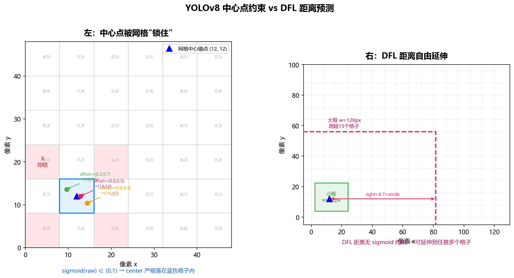
第一部分:中心点为什么被网格"锁住"
YOLOv8 在每一层特征图上铺了一张均匀网格。以 P3 层为例,输入图像 640×640 被划分成 80×80 = 6400 个格子,每个格子对应 8×8 像素的区域(8 就是这层的步长 stride)。
模型对每个格子输出两个原始值——我们叫它 raw_cx 和 raw_cy。但这两个值不能直接当坐标用,它们会先经过一次 sigmoid 函数:
offset_x = sigmoid(raw_cx)   # 结果在 (0, 1) 之间
offset_y = sigmoid(raw_cy)   # 结果在 (0, 1) 之间
sigmoid 的值域是 (0, 1),永远不会等于 0 也不会等于 1。这意味着偏移量被严格压缩在"不到一个格子"的范围内。最终的中心点坐标通过以下公式还原:
实际中心x = (grid_j + offset_x) × stride
实际中心y = (grid_i + offset_y) × stride
这里 grid_j 和 grid_i 是网格列号和行号(整数),offset_x/y 是 0 到 1 之间的小数。所以最终的中心点坐标一定落在 grid_j × stride 到 (grid_j + 1) × stride 这个区间内——也就是严格在自己所属的那个格子里,绝对跑不到隔壁格子去。
举个具体的数值例子:网格第 1 行第 1 列(索引从 0 开始),stride = 8。如果模型输出的 sigmoid 偏移是 (0.6, 0.5),那么:
cx = (1 + 0.6) × 8 = 12.8 像素
cy = (1 + 0.5) × 8 = 12.0 像素
这个中心点一定落在 8~16 像素的范围内(第 1 列格子的区域),即使模型"想让它偏更远",sigmoid 也不允许偏移超过 1.0。
这就是"中心点被网格约束"的具体含义——网格决定了中心点的大致位置(哪个 8×8 区域),sigmoid 只允许在这个区域内微调精确位置。
代码实现:make_anchors — 固定锚点位于格子中心
YOLOv8 通过 make_anchors 函数生成每个格子的中心锚点坐标(特征图坐标系),默认偏移 grid_cell_offset=0.5,使锚点恰好在格子中央。
def make_anchors(feats, strides, grid_cell_offset=0.5):
    """Generate anchors from features."""
    anchor_points, stride_tensor = [], []
    assert feats is not None
    dtype, device = feats[0].dtype, feats[0].device
    for i in range(len(feats)):
        stride = strides[i]
        h, w = feats[i].shape[2:] if isinstance(feats, list) else (int(feats[i][0]), int(feats[i][1]))
        sx = torch.arange(end=w, device=device, dtype=dtype) + grid_cell_offset  # shift x
        sy = torch.arange(end=h, device=device, dtype=dtype) + grid_cell_offset  # shift y
        sy, sx = torch.meshgrid(sy, sx, indexing="ij") if TORCH_1_11 else torch.meshgrid(sy, sx)
        anchor_points.append(torch.stack((sx, sy), -1).view(-1, 2))
        stride_tensor.append(torch.full((h * w, 1), stride, dtype=dtype, device=device))
return torch.cat(anchor_points), torch.cat(stride_tensor)关键细节:
-
sx = torch.arange(end=w) + 0.5:第 j 列格子的锚点 x 坐标 =j + 0.5(特征图坐标),乘以 stride 后 =(j + 0.5) × stride,精确落在格子中央。 -
stride_tensor存储每个锚点对应的 stride,用于后续坐标还原到图像尺寸。 -
该函数在推理路径的
_get_decode_boxes(head.py:179)中被调用:
# head.py:175-182
def _get_decode_boxes(self, x: dict[str, torch.Tensor]) -> torch.Tensor:
    """Get decoded boxes based on anchors and strides."""
    shape = x["feats"][0].shape  # BCHW
    if self.dynamic or self.shape != shape:
        self.anchors, self.strides = (a.transpose(0, 1) for a in make_anchors(x["feats"], self.stride, 0.5))
        self.shape = shape

    dbox = self.decode_bboxes(self.dfl(x["boxes"]), self.anchors.unsqueeze(0)) * self.strides
return dbox注:YOLOv8 采用 无锚框(anchor-free) 的 DFL 解码机制。"中心点被约束在格子内"这一效果,在 YOLOv8 中并非通过对偏移量直接施加 sigmoid 实现,而是通过任务对齐标签分配(TAL)在训练时将目标锚点固定为离目标中心最近的格子中心点,再结合 DFL 的距离预测来间接实现的。概念上与上述 sigmoid 机制等价:每个格子只负责预测以自身中心为锚点的那些目标。
第二部分:宽高为什么不受约束
中心点确定后,接下来要确定边界框有多大。这里 YOLOv8 用的不是传统的直接预测 w 和 h,而是通过 DFL(Distributed Focal Loss,分布焦点损失)机制,预测中心点到四条边的距离:top、bottom、left、right。
关键区别在于:这四个距离值不经过 sigmoid 处理。
DFL 的工作方式是把连续的距离值离散化为一组整数刻度(默认是 0~15,共 16 个 bin),模型输出的是这 16 个刻度的概率分布,然后通过加权求和得到最终的距离预测值。这个求和结果是一个连续的浮点数,理论范围是 0 到 15(单位是 stride),没有上下界的硬约束。
最终的宽高还原方式:
w = (dist_left + dist_right) × stride
h = (dist_top + dist_bottom) × stride
以 P3 层 stride=8 为例,如果模型预测 left=6.3、right=8.7,那么:
w = (6.3 + 8.7) × 8 = 120 像素
120 像素跨越了 15 个网格格子——远远超出了中心点所在的那个 8×8 的小格子。这就是为什么"一个小网格点也能预测出一个大框"。
再极端一点,如果 left 和 right 都接近最大值 15,那么:
w = (15 + 15) × 8 = 240 像素
一个 P3 层的网格点可以预测出宽度达 240 像素的框,覆盖将近输入图像三分之一的宽度。
代码实现:DFL 模块 — 概率分布到期望距离
class DFL(nn.Module):
"""Integral module of Distribution Focal Loss (DFL).
Proposed in Generalized Focal Loss https://ieeexplore.ieee.org/document/9792391
"""
def __init__(self, c1: int = 16):
super().__init__()
self.conv = nn.Conv2d(c1, 1, 1, bias=False).requires_grad_(False)
x = torch.arange(c1, dtype=torch.float)
self.conv.weight.data[:] = nn.Parameter(x.view(1, c1, 1, 1)) # 权重固定为 [0,1,...,15]
self.c1 = c1
def forward(self, x: torch.Tensor) -> torch.Tensor:
"""Apply the DFL module to input tensor and return transformed output."""
b, _, a = x.shape # batch, channels, anchors
return self.conv(x.view(b, 4, self.c1, a).transpose(2, 1).softmax(1)).view(b, 4, a)逐步解读 forward:
| 步骤 | 操作 | 张量形状 | 含义 |
|---|---|---|---|
| 输入 | x |
(b, 4×16, n) |
每个锚点 4 个方向 × 16 个 bin 的原始 logits |
| reshape | view(b, 4, 16, n) |
(b, 4, 16, n) |
拆分为 4 个方向 |
| transpose | transpose(2, 1) |
(b, 16, 4, n) |
将 bin 维移到 channel 维 |
| softmax | softmax(dim=1) |
(b, 16, 4, n) |
对 16 个 bin 归一化为概率(无 sigmoid!) |
| conv | conv(...) |
(b, 1, 4, n) |
与权重 [0,1,...,15] 点积 = 加权期望 |
| 输出 | view(b, 4, n) |
(b, 4, n) |
4 个方向的距离预测(单位:stride 格子数) |
核心操作是 softmax + conv(权重固定为 [0,1,...,15]),本质是计算概率分布的期望值: $$\hat{d} = \sum_{i=0}^{15} p_i \cdot i$$
其中 $p_i$ 是第 $i$ 个 bin 的 softmax 概率。结果 $\hat{d} \in (0, 15)$,无上界硬约束。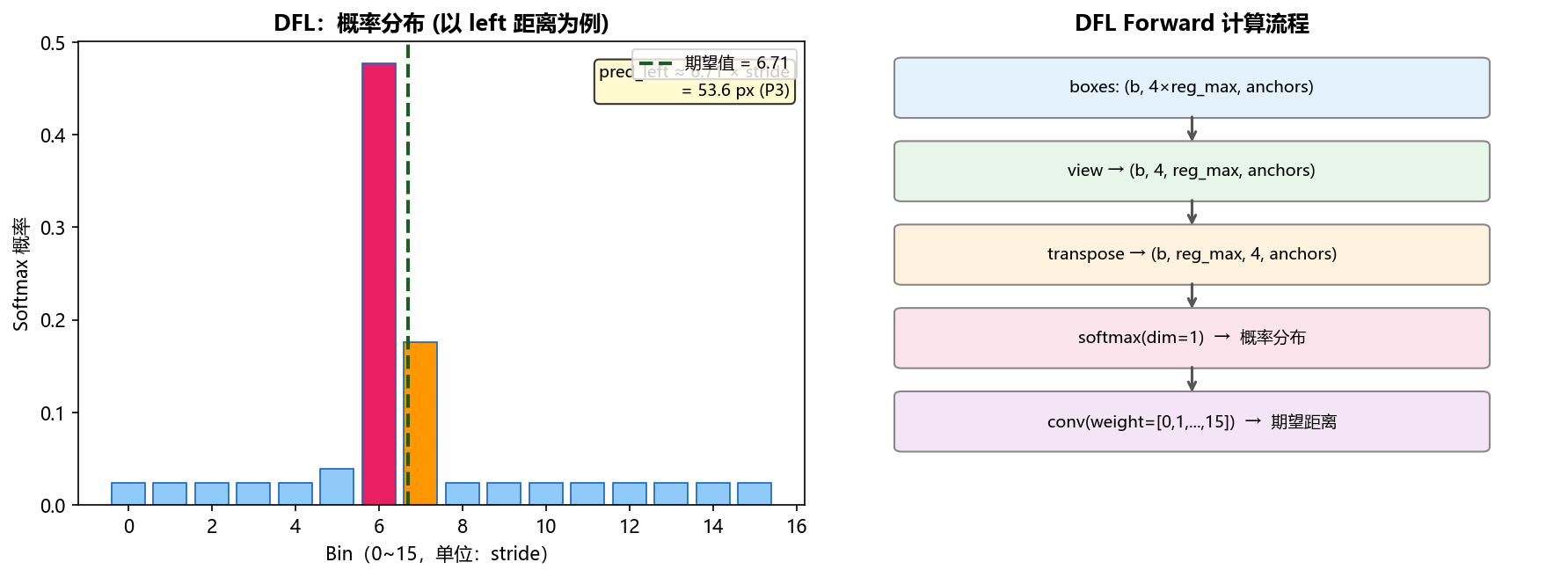
代码实现:dist2bbox — 距离转换为边界框坐标
def dist2bbox(distance, anchor_points, xywh=True, dim=-1):
    """Transform distance(ltrb) to box(xywh or xyxy)."""
    lt, rb = distance.chunk(2, dim)      # left/top 和 right/bottom
    x1y1 = anchor_points - lt           # 左上角 = 锚点 - 左/上距离
    x2y2 = anchor_points + rb           # 右下角 = 锚点 + 右/下距离
    if xywh:
        c_xy = (x1y1 + x2y2) / 2        # 中心坐标
        wh = x2y2 - x1y1                # 宽高 = (left+right, top+bottom)
        return torch.cat([c_xy, wh], dim)  # xywh bbox
return torch.cat((x1y1, x2y2), dim) # xyxy bbox这里宽高的计算方式说明了"无约束"的本质:
w = (dist_left + dist_right)     # 单位:特征图格子数
h = (dist_top  + dist_bottom)
乘以 stride 后得到图像像素坐标,没有任何 sigmoid 或 clamp 限制(训练时有 clamp_(0, reg_max-0.01) 但仅用于稳定梯度)。
代码实现:训练时的 DFL Loss
class DFLoss(nn.Module):
"""Criterion class for computing Distribution Focal Loss (DFL)."""
def __init__(self, reg_max: int = 16) -> None:
super().__init__()
self.reg_max = reg_max
def __call__(self, pred_dist: torch.Tensor, target: torch.Tensor) -> torch.Tensor:
"""Return sum of left and right DFL losses."""
target = target.clamp_(0, self.reg_max - 1 - 0.01) # 截断到 [0, 14.99]
tl = target.long() # target left bin
tr = tl + 1 # target right bin
wl = tr - target # 左 bin 的插值权重
wr = 1 - wl # 右 bin 的插值权重
return (
F.cross_entropy(pred_dist, tl.view(-1), reduction="none").view(tl.shape) * wl
+ F.cross_entropy(pred_dist, tr.view(-1), reduction="none").view(tl.shape) * wr
).mean(-1, keepdim=True)关键设计:
-
clamp_(0, reg_max - 1 - 0.01):训练目标限制在[0, 14.99],用两个相邻整数 bin 做插值,实现软标签监督。 -
并非对距离本身加上界,而是对监督目标加约束,推理时距离值仍可超出(但会超出分布支持范围而损失较大)。
代码实现:推理时解码流程
def bbox_decode(self, anchor_points: torch.Tensor, pred_dist: torch.Tensor) -> torch.Tensor:
    """Decode predicted object bounding box coordinates from anchor points and distribution."""
    if self.use_dfl:
        b, a, c = pred_dist.shape  # batch, anchors, channels
        pred_dist = pred_dist.view(b, a, 4, c // 4).softmax(3).matmul(self.proj.type(pred_dist.dtype))
        # self.proj = torch.arange(reg_max)  即 [0, 1, ..., 15]
    return dist2bbox(pred_dist, anchor_points, xywh=False)
第三部分:为什么要这样设计
这两种不同的约束策略背后有清晰的工程理由。
对中心点施加 sigmoid 约束(或通过 TAL 锚点分配实现等价效果),是为了避免多个网格点争抢同一个目标。如果中心点可以随意漂移到其他格子的区域,那么相邻的多个格子都可能把中心点预测到同一个目标上,造成更严重的重复检测,增加 NMS 的负担。约束中心点之后,每个目标的中心点只会被一个(或少数几个相邻的)格子负责预测,重复率会大幅降低。
对宽高不施加约束,是为了让模型有能力检测各种尺度的目标。虽然不同的特征层(P3/P4/P5)分别负责不同尺度的目标,但实际场景中目标大小的分布并不会严格落在设计好的尺度区间内。放开宽高约束,让每个网格点都有能力"向外伸展"去覆盖更大的区域,提高了模型对各种尺寸目标的适应能力。
简单总结:中心点用约束是为了"谁负责谁"的归属问题,宽高不约束是为了"能检测多大"的能力问题。这两个设计目标本质上是解耦的,所以采用了不同的处理策略。
完整推理解码流程图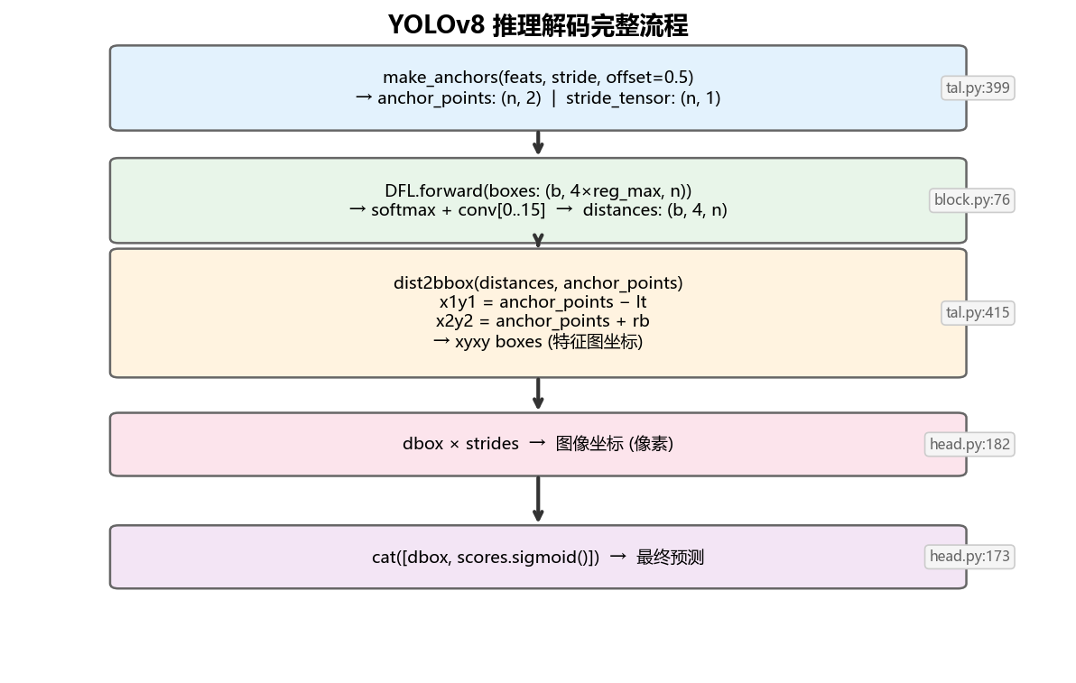
| 步骤 | 代码位置 | 核心操作 |
|---|---|---|
| 1. 生成锚点 | tal.py:399 |
make_anchors(feats, stride, 0.5) → 每格中心坐标 |
| 2. DFL 解码距离 | block.py:76 |
softmax + conv[0..15] → ltrb 距离(无 sigmoid) |
| 3. 距离转框 | tal.py:415 |
dist2bbox → xyxy 坐标(特征图坐标) |
| 4. 缩放到图像 | head.py:182 |
dbox × strides → 像素坐标 |
| 5. 分类概率 | head.py:173 |
scores.sigmoid() → 类别置信度 |
附录:关键超参数对比
| 参数 | YOLOv8 默认值 | YOLO26 值 | 含义 | 代码位置 |
|---|---|---|---|---|
reg_max |
16 | 1 | DFL bin 数量;=1 时 DFL 退化为 Identity | head.py:90 |
end2end |
False | True | 是否启用双头端到端设计 | head.py:111 |
grid_cell_offset |
0.5 | 0.5(不变) | 锚点相对格子左上角的偏移(0.5 = 格子中心) | tal.py:399 |
stride |
[8, 16, 32] | [8, 16, 32](不变) | P3/P4/P5 层步长 | 模型配置 |
xywh in decode_bboxes |
True | False(端到端强制) | bbox 输出格式 | head.py:204 |
-
YOLOv8 P3 层(stride=8)单点最大可预测框宽 =
(15 + 15) × 8 = 240px(37.5% 图像宽) -
YOLO26
reg_max=1,距离为直接回归值,理论无上界(由训练数据分布和 loss 隐式约束)
YOLO26 的无锚框设计
YOLO26 在 YOLOv8 无锚框体系的基础上进行了进一步演进,核心变化集中在两点:去除 DFL 分布建模(reg_max=1) 和 引入端到端双头设计(end2end=True)。两者共同使模型在保持无锚框定位优势的同时,显著降低推理复杂度并消除 NMS 依赖。
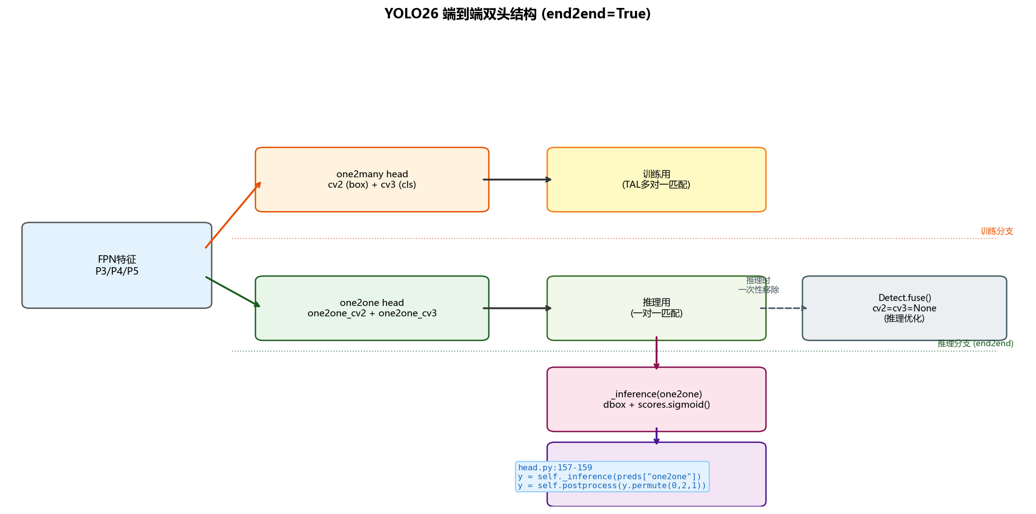
4.1 架构总览
下图展示了两代模型的完整解码流程对比: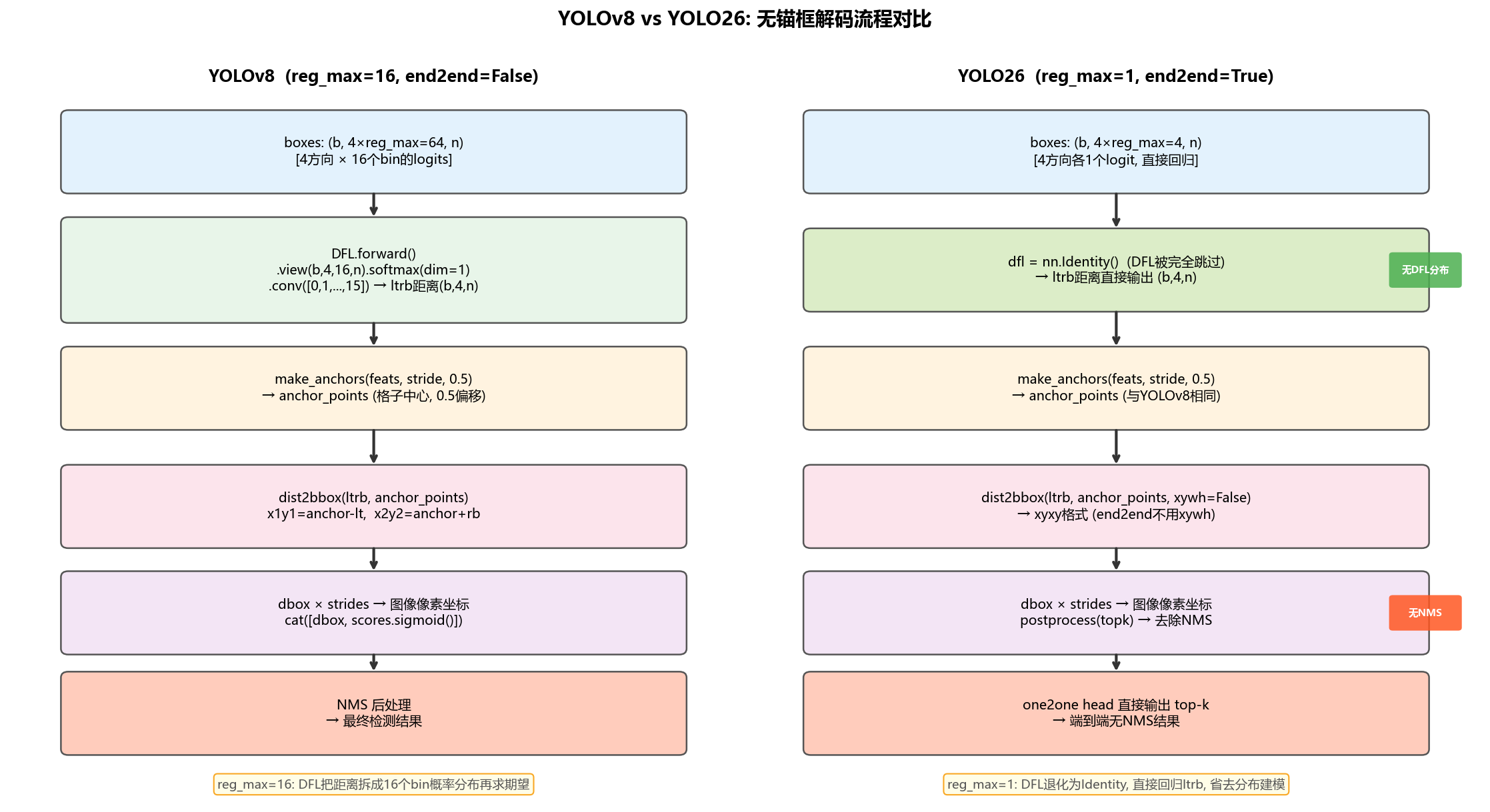
4.2 关键改动一:reg_max=1,DFL 退化为 Identity
YOLOv8 用 DFL 把每个方向的距离建模为 16 个 bin 的概率分布(reg_max=16),通过加权期望得到连续距离值。YOLO26 将 reg_max 设为 1,DFL 模块被彻底绕过:
# yolo26.yaml
nc: 80
end2end: True    # 端到端模式
reg_max: 1       # DFL bins = 1,即不用DFL
触发逻辑在检测头初始化处:
# Detect.__init__
self.reg_max = reg_max # YOLO26 中 = 1
self.no = nc + self.reg_max * 4 # 每锚点输出数 = nc + 4(不再是 nc + 64)
self.dfl = DFL(self.reg_max) if self.reg_max > 1 else nn.Identity()
# ^^^^^^^^^^^^^^^^
# reg_max=1 时 DFL 被替换为 Identity,boxes 直接透传cv2 分支输出从 (b, 4×16, n) 缩减为 (b, 4×1, n) = (b, 4, n),每个锚点直接输出 4 个标量距离(ltrb),而非 64 个 logits。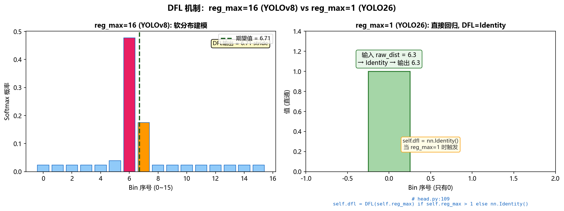
效果:
| 对比项 | YOLOv8 | YOLO26 |
|---|---|---|
| box 分支输出通道 | 4 × 16 = 64 |
4 × 1 = 4 |
| DFL 运算 | softmax + 卷积期望 | nn.Identity() 直通 |
| 距离精度 | 软分布建模,次像素精度 | 直接回归,梯度更直接 |
| 参数量影响 | 较多 | 减少(cv2 更轻量) |
4.3 关键改动二:end2end=True,双头无 NMS
YOLO26 在检测头中同时维护两个并行分支:
-
one2many head(
cv2/cv3):训练时启用,传统一对多匹配,提供丰富梯度信号 -
one2one head(
one2one_cv2/one2one_cv3):推理时启用,一对一匹配,输出无冗余,无需 NMS
# Detect.__init__:当 end2end=True 时复制出 one2one 分支
if end2end:
self.one2one_cv2 = copy.deepcopy(self.cv2)
self.one2one_cv3 = copy.deepcopy(self.cv3)
# Detect.forward:训练用两个头,推理只用 one2one
def forward(self, x):
preds = self.forward_head(x, **self.one2many) # one2many 分支
if self.end2end:
x_detach = [xi.detach() for xi in x]
one2one = self.forward_head(x_detach, **self.one2one) # one2one 分支
preds = {"one2many": preds, "one2one": one2one}
if self.training:
return preds # 训练:返回两组原始预测
y = self._inference(preds["one2one"] if self.end2end else preds)
if self.end2end:
y = self.postprocess(y.permute(0, 2, 1)) # 推理:topk 替代 NMS
return y if self.export else (y, preds)推理时 postprocess 替代 NMS:
def postprocess(self, preds: torch.Tensor) -> torch.Tensor:
    """Post-processes YOLO model predictions."""
    boxes, scores = preds.split([4, self.nc], dim=-1)
    scores, conf, idx = self.get_topk_index(scores, self.max_det)
    boxes = boxes.gather(dim=1, index=idx.repeat(1, 1, 4))
    return torch.cat([boxes, scores, conf], dim=-1)
# 直接 top-k 选取,无 IoU 阈值过滤,无排序+suppression推理优化:fuse() 抹去 one2many 头:
decode_bboxes 的 xywh 参数随之改变:

# head.py:199-206
def decode_bboxes(self, bboxes, anchors, xywh=True):
    return dist2bbox(
        bboxes,
        anchors,
        xywh=xywh and not self.end2end and not self.xyxy,  # end2end 时强制 xyxy
        dim=1,
    )
YOLOv8 默认返回 xywh 格式便于损失计算;YOLO26 因 end2end=True,直接返回 xyxy 格式交给 postprocess。
4.4 扩展头:OBB26、Segment26、Pose26
YOLO26 对多任务头也做了针对性改动:
OBB26:去除角度 sigmoid
class OBB26(OBB):
"""输出原始角度 logits,不经过 sigmoid 变换"""
def forward_head(self, x, box_head, cls_head, angle_head):
preds = Detect.forward_head(self, x, box_head, cls_head)
if angle_head is not None:
bs = x[0].shape[0]
angle = torch.cat(
[angle_head[i](x[i]).view(bs, self.ne, -1) for i in range(self.nl)], 2
) # OBB theta logits(raw output without sigmoid transformation)
preds["angle"] = angle
return preds标准 OBB 在推理时对角度施加 sigmoid 将其映射到 [-π/4, 3π/4],YOLO26 OBB26 跳过此操作,输出原始 logits,避免在 ±π/4 等边界处出现梯度消失。
Segment26:多尺度原型融合
class Segment26(Segment):
def __init__(self, ...):
super().__init__(...)
self.proto = Proto26(ch, self.npr, self.nm, nc) # 替换标准 Proto
Proto26 在标准原型网络基础上增加了多尺度特征融合和语义分割辅助分支:
class Proto26(Proto):
def __init__(self, ch, c_, c2, nc):
super().__init__(c_, c_, c2)
self.feat_refine = nn.ModuleList(Conv(x, ch[0], k=1) for x in ch[1:]) # P4,P5→P3分辨率
self.feat_fuse = Conv(ch[0], c_, k=3)
self.semseg = nn.Sequential(Conv(ch[0], c_, k=3), Conv(c_, c_, k=3), nn.Conv2d(c_, nc, 1))
def forward(self, x, return_semseg=True):
feat = x[0] # P3 最高分辨率特征
for i, f in enumerate(self.feat_refine):
up_feat = f(x[i + 1]) # 将 P4/P5 通道对齐到 P3
up_feat = F.interpolate(up_feat, size=feat.shape[2:], mode="nearest")
feat = feat + up_feat # 多尺度累加融合
p = super().forward(self.feat_fuse(feat))
if self.training and return_semseg:
semseg = self.semseg(feat)
return (p, semseg) # 训练时额外返回语义分割图
return pPose26:RealNVP 归一化流 + 不确定性估计
class Pose26(Pose):
    def __init__(self, ...):
        super().__init__(...)
        self.flow_model = RealNVP()             # 归一化流用于关键点分布建模
        self.cv4_sigma = nn.ModuleList(...)     # 每个关键点预测 (σ_x, σ_y) 不确定性
RealNVP 通过可逆变换把关键点的复杂分布映射到标准高斯分布,用于更精确的似然估计和训练监督。kpts_decode 中关键点坐标用直接加法而非缩放 sigmoid:
# Pose26.kpts_decode (head.py:767-768)
y[:, 0::ndim] = (y[:, 0::ndim] + self.anchors[0]) * self.strides   # x = (raw + anchor) × stride
y[:, 1::ndim] = (y[:, 1::ndim] + self.anchors[1]) * self.strides   # y = (raw + anchor) × stride
# 对比标准 Pose: (raw * 2.0 + anchor - 0.5) × stride,YOLO26 去掉了 *2 和 -0.5 的缩放
4.5 YOLO26 vs YOLOv8 设计差异总结
| 设计维度 | YOLOv8 | YOLO26 |
|---|---|---|
reg_max |
16 | 1 |
| DFL 机制 | softmax + 加权求和 | nn.Identity()(直接回归) |
| 检测头数量 | 1 个(one2many) | 2 个(one2many + one2one) |
| 后处理 | NMS(IoU 阈值) | topk postprocess(无 NMS) |
推理时 fuse() |
移除 one2many(若 end2end) | 同左,cv2/cv3 置 None |
| bbox 输出格式 | xywh(训练) | xyxy(end2end 强制) |
| 角度预测(OBB) | sigmoid 映射到 [-π/4, 3π/4] | 原始 logits,无 sigmoid |
| 分割原型(Seg) | 单尺度 Proto | 多尺度融合 Proto26 + 语义分割辅助 |
| 关键点(Pose) | 直接回归 + sigmoid(vis) | RealNVP 流 + σ 不确定性估计 |
设计哲学:YOLO26 用直接回归替代分布建模(去 DFL),用一对一匹配替代 NMS(end2end),在保持无锚框空间灵活性的同时,以更简洁的解码路径换取推理效率提升。两代模型的无锚框本质(
make_anchors+dist2bbox)保持不变。

腾讯云面向开发者汇聚海量精品云计算使用和开发经验,营造开放的云计算技术生态圈。
更多推荐
 5
5 0
0- 0


 已为社区贡献1条内容

所有评论(0)