---

一、顶层架构：边缘检测的本质

1.1 数学基础：从连续到离散

连续空间：边缘 = 亮度函数的突变点
           ↓ 离散化
数字图像：边缘 = 相邻像素的剧烈变化
           ↓ 数学工具
        微分/差分 ≈ 变化率

1.2 检测策略的两大分支

图像边缘检测 → 两种核心思路
├── 基于一阶梯度：寻找"坡度最大值"
│   ├── 物理意义：地形中最陡峭处
│   └── 代表：Sobel、Scharr → Canny
│
└── 基于二阶梯度：寻找"坡度变化零点"
    ├── 物理意义：从陡变缓的转折点
    └── 代表：Laplacian

---

二、一阶梯度方法：寻找最大变化率

2.1 核心原理

第一性原理：f'(x) ≈ Δf/Δx ≈ 相邻像素差值
数值实现：卷积核滑动计算
关键输出：梯度幅值(陡峭程度) + 梯度方向(边缘朝向)

2.2 Sobel 算子：平衡的艺术

演进逻辑：
简单差分[-1, 1] → 噪声敏感 → 需要平滑
    ↓
Sobel核设计：
Gx = [[-1, 0, 1],     Gy = [[-1, -2, -1],
      [-2, 0, 2],           [ 0,  0,  0],
      [-1, 0, 1]]           [ 1,  2,  1]]

设计智慧：
1. 中心行/列权重×2 → 差分+垂直方向平滑
2. 3×3窗口 → 局部平均降噪
3. 分离性 → 计算高效

2.3 Scharr 算子：旋转对称性优化

Sobel的局限：对角边缘响应不足
    ↓
Scharr改进：
Gx = [[-3, 0,  3],    Gy = [[-3, -10, -3],
      [-10,0, 10],          [ 0,   0,  0],
      [-3, 0,  3]]          [ 3,  10,  3]]

优化点：
1. 更大的中心权重(10 vs 2)
2. 更好的旋转对称性
3. 45°方向误差减少30-50%

---

三、二阶梯度方法：Laplacian 的得与失

3.1 数学本质

连续Laplacian：∇²f = ∂²f/∂x² + ∂²f/∂y²
离散近似：4-邻域核 [[0,1,0],[1,-4,1],[0,1,0]]
             或8-邻域核 [[1,1,1],[1,-8,1],[1,1,1]]

3.2 关键特性分析

优点：
1. 各向同性 → 旋转不变，所有方向同等对待
2. 零交叉定位 → 理论上边缘定位更精确
3. 无方向性 → 无需计算梯度方向

致命缺点：噪声放大效应
二阶微分 → 对高频分量加倍响应
          ↓
    噪声被严重放大
          ↓
  需要先进行强力平滑

3.3 实际应用形式

为解决噪声问题，实际常用：
1. Laplacian of Gaussian (LoG)
   高斯平滑 + Laplacian → 先降噪再求二阶导
    
2. Difference of Gaussians (DoG)
   两个不同σ的高斯核差值 → LoG的近似但更高效

---

四、集大成者：Canny 边缘检测器

4.1 设计哲学：模拟人类视觉

人类视觉特性            → Canny对应步骤
1. 自动降噪             → 高斯模糊
2. 对比度增强           → 梯度计算
3. 轮廓细化             → 非极大值抑制
4. 感知连续性           → 双阈值连接

4.2 四步流程详解

步骤 1：高斯模糊 - 噪声防火墙

核函数：G(x,y) = (1/(2πσ²))·exp(-(x²+y²)/(2σ²))
σ选择：平衡平滑与定位精度
  小σ(0.5-1.5) → 细节保留好，噪声抑制弱
  大σ(1.5-3.0) → 噪声抑制强，边缘模糊

步骤 2：梯度计算 - 变化率测量

可选用算子：
          | 精度 | 抗噪性 | 计算量 | 适用场景
Sobel     | 中   | 良     | 低     | 实时应用
Scharr    | 高   | 良     | 中     | 高精度需求

步骤 3：非极大值抑制 - 边缘细化

算法流程：
for 每个像素点p:
    1. 获取梯度方向θ
    2. 沿θ方向找到两个相邻像素q,r
    3. if p的梯度值 < q或r的梯度值:
           将p抑制为0(非边缘)
       else:
           保留p为候选边缘点
    
方向离散化(典型实现):
   0°   → 水平方向比较
   45°  → 对角线比较
   90°  → 垂直方向比较
   135° → 另一对角线比较

步骤 4：双阈值滞后连接 - 智能决策

阈值设定原则：
高阈值Thigh ≈ 图像梯度幅值直方图的前30%
低阈值Tlow  ≈ 0.4-0.5 × Thigh

连接算法伪代码：
1. 初始化: strong_edges = [], weak_edges = []
2. 第一次扫描:
   if 梯度值 > Thigh: 标记为强边缘，加入strong_edges
   elif 梯度值 > Tlow: 标记为弱边缘，加入weak_edges
   else: 标记为非边缘
3. 第二次扫描(连接):
   for 每个弱边缘像素p:
       if p的8邻域中存在强边缘像素:
           将p升级为强边缘
       else:
           将p降级为非边缘

---

五、算法对比与选择指南

5.1 性能比较矩阵

算法/特性	边缘连续性	抗噪性	定位精度	计算复杂度	单像素宽
Sobel	差	中	中	低	否
Scharr	差	中	高	中	否
Laplacian	差	差	高(理论)	低	是
Canny	优	优	高	高	是

5.2 应用场景建议

实时视频处理 → Sobel(简单快速)
精密测量系统 → Scharr(精度优先)
理论分析研究 → Laplacian + Gaussian
通用工业检测 → Canny(调整参数σ,阈值)
资源受限环境 → 简化Canny(跳过部分步骤)

5.3 参数调优经验值

Canny参数初始值：
σ = 1.0-1.5 (适中平滑)
Thigh = 梯度幅值直方图70%分位数
Tlow = 0.4 × Thigh

调优方向：
更多细节 → 减小σ，降低阈值
更强降噪 → 增大σ，提高阈值

---

六、演进脉络总结

6.1 历史发展轴线

1960s: 简单差分算子
1970:  Sobel引入平滑思想
1970s: Laplacian理论完善
1980s: Marr提出LoG，Canny提出完整框架
1990s: Canny成为工业标准
2000s+: 深度学习边缘检测兴起

6.2 核心思想演进

1. 从"变化"到"最优变化检测"
   Sobel → 考虑局部平均
   
2. 从"单步"到"流程化"
   简单算子 → Canny多阶段优化
   
3. 从"手工设计"到"数据驱动"
   传统算子 → 深度学习特征学习

6.3 现代扩展与变种

实时Canny: 积分图像加速
自适应Canny: 局部阈值调整
彩色Canny: 多通道梯度融合
深度学习: HED, RCF等端到端边缘检测

七、实战演练-Python代码

import numpy as np
import cv2
import matplotlib.pyplot as plt

# 设置中文字体支持
plt.rcParams['font.sans-serif'] = ['SimHei']
plt.rcParams['axes.unicode_minus'] = False


# 1. 创建测试图像 - 简单的棋盘格
def create_chessboard(size=200, square_size=20):
    """创建棋盘格测试图像"""
    chessboard = np.zeros((size, size), dtype=np.uint8)

    for i in range(0, size, square_size):
        for j in range(0, size, square_size):
            if (i // square_size + j // square_size) % 2 == 0:
                chessboard[i:i + square_size, j:j + square_size] = 255

    return chessboard


# 2. 创建带噪声的棋盘格（用于测试抗噪性）
def add_noise(image, noise_level=0.1):
    """添加椒盐噪声"""
    noisy = image.copy()
    h, w = image.shape
    num_noise = int(noise_level * h * w)

    for _ in range(num_noise):
        x = np.random.randint(0, h)
        y = np.random.randint(0, w)
        noisy[x, y] = 255 if np.random.random() > 0.5 else 0

    return noisy


# 3. 边缘检测函数集
def apply_sobel(image):
    """Sobel边缘检测"""
    sobel_x = cv2.Sobel(image, cv2.CV_64F, 1, 0, ksize=3)
    sobel_y = cv2.Sobel(image, cv2.CV_64F, 0, 1, ksize=3)
    sobel = np.sqrt(sobel_x ** 2 + sobel_y ** 2)
    return np.uint8(np.clip(sobel, 0, 255))


def apply_scharr(image):
    """Scharr边缘检测"""
    scharr_x = cv2.Scharr(image, cv2.CV_64F, 1, 0)
    scharr_y = cv2.Scharr(image, cv2.CV_64F, 0, 1)
    scharr = np.sqrt(scharr_x ** 2 + scharr_y ** 2)
    return np.uint8(np.clip(scharr, 0, 255))


def apply_laplacian(image):
    """Laplacian边缘检测"""
    laplacian = cv2.Laplacian(image, cv2.CV_64F)
    laplacian_abs = np.absolute(laplacian)
    return np.uint8(np.clip(laplacian_abs, 0, 255))


def apply_canny(image, low_threshold=50, high_threshold=150):
    """Canny边缘检测"""
    return cv2.Canny(image, low_threshold, high_threshold)


def apply_log(image, sigma=1.0):
    """LoG(Laplacian of Gaussian)边缘检测"""
    # 先高斯模糊
    blurred = cv2.GaussianBlur(image, (5, 5), sigma)
    # 再Laplacian
    laplacian = cv2.Laplacian(blurred, cv2.CV_64F)
    laplacian_abs = np.absolute(laplacian)
    return np.uint8(np.clip(laplacian_abs, 0, 255))


# 4. 创建可视化对比图
def visualize_comparison(original, noisy, results, titles):
    """可视化原始图像、噪声图像和各算法结果"""
    fig, axes = plt.subplots(2, 4, figsize=(16, 8))

    # 第一行：原始图像和各算法在干净图像上的结果
    axes[0, 0].imshow(original, cmap='gray')
    axes[0, 0].set_title('原始棋盘格图像')
    axes[0, 0].axis('off')

    for i in range(1, 4):
        axes[0, i].imshow(results[i - 1], cmap='gray')
        axes[0, i].set_title(titles[i - 1])
        axes[0, i].axis('off')

    # 第二行：噪声图像和各算法在噪声图像上的结果
    axes[1, 0].imshow(noisy, cmap='gray')
    axes[1, 0].set_title('添加噪声的图像')
    axes[1, 0].axis('off')

    for i in range(1, 4):
        axes[1, i].imshow(results[i + 2], cmap='gray')
        axes[1, i].set_title(titles[i + 2] + " (噪声)")
        axes[1, i].axis('off')

    plt.tight_layout()
    plt.show()


# 5. 创建算法步骤分解图（Canny示例）
def visualize_canny_steps(image):
    """可视化Canny算法的每个步骤"""
    # 步骤1: 高斯模糊
    blurred = cv2.GaussianBlur(image, (5, 5), 1.0)

    # 步骤2: 梯度计算（使用Sobel）
    grad_x = cv2.Sobel(blurred, cv2.CV_64F, 1, 0, ksize=3)
    grad_y = cv2.Sobel(blurred, cv2.CV_64F, 0, 1, ksize=3)
    magnitude = np.sqrt(grad_x ** 2 + grad_y ** 2)
    direction = np.arctan2(grad_y, grad_x) * 180 / np.pi

    # 步骤3: 非极大值抑制（简化实现）
    def non_maximum_suppression(mag, angle):
        h, w = mag.shape
        suppressed = np.zeros((h, w), dtype=np.float32)

        for i in range(1, h - 1):
            for j in range(1, w - 1):
                # 将角度量化到4个方向
                if (0 <= angle[i, j] < 22.5) or (157.5 <= angle[i, j] <= 180) or (-22.5 <= angle[i, j] < 0) or (
                        -180 <= angle[i, j] < -157.5):
                    # 水平方向
                    neighbors = [mag[i, j - 1], mag[i, j + 1]]
                elif (22.5 <= angle[i, j] < 67.5) or (-157.5 <= angle[i, j] < -112.5):
                    # 45度方向
                    neighbors = [mag[i - 1, j - 1], mag[i + 1, j + 1]]
                elif (67.5 <= angle[i, j] < 112.5) or (-112.5 <= angle[i, j] < -67.5):
                    # 垂直方向
                    neighbors = [mag[i - 1, j], mag[i + 1, j]]
                else:
                    # 135度方向
                    neighbors = [mag[i - 1, j + 1], mag[i + 1, j - 1]]

                if mag[i, j] >= max(neighbors):
                    suppressed[i, j] = mag[i, j]

        return suppressed

    nms = non_maximum_suppression(magnitude, direction)

    # 步骤4: 双阈值处理
    high_threshold = 50
    low_threshold = 20

    strong_edges = (nms > high_threshold)
    weak_edges = (nms >= low_threshold) & (nms <= high_threshold)

    # 最终结果
    final_edges = np.zeros_like(image, dtype=np.uint8)
    final_edges[strong_edges] = 255

    # 可视化
    fig, axes = plt.subplots(2, 3, figsize=(15, 10))

    steps = [
        (image, '原始图像'),
        (blurred, '1. 高斯模糊后'),
        (np.uint8(np.clip(magnitude, 0, 255)), '2. 梯度幅值图'),
        (np.uint8(np.clip(nms, 0, 255)), '3. 非极大值抑制后'),
        (np.uint8(weak_edges * 255), '弱边缘（阈值间）'),
        (final_edges, '4. 最终Canny边缘')
    ]

    for idx, (img, title) in enumerate(steps):
        ax = axes[idx // 3, idx % 3]
        ax.imshow(img, cmap='gray')
        ax.set_title(title)
        ax.axis('off')

    plt.tight_layout()
    plt.show()


# 6. 执行演示
if __name__ == "__main__":
    print("=== 图像边缘检测算法演示 ===\n")

    # 创建测试图像
    print("1. 创建棋盘格测试图像...")
    chessboard = create_chessboard(200, 20)
    noisy_chessboard = add_noise(chessboard, 0.05)

    # 应用各种边缘检测算法
    print("2. 应用各种边缘检测算法...")

    # 在干净图像上的结果
    sobel_result = apply_sobel(chessboard)
    scharr_result = apply_scharr(chessboard)
    canny_result = apply_canny(chessboard, 30, 100)

    # 在噪声图像上的结果
    sobel_noisy = apply_sobel(noisy_chessboard)
    laplacian_noisy = apply_laplacian(noisy_chessboard)
    canny_noisy = apply_canny(noisy_chessboard, 30, 100)
    log_noisy = apply_log(noisy_chessboard, 1.5)

    # 准备可视化
    clean_results = [sobel_result, scharr_result, canny_result]
    clean_titles = ['Sobel边缘检测', 'Scharr边缘检测', 'Canny边缘检测']

    noisy_results = [sobel_noisy, laplacian_noisy, canny_noisy, log_noisy]
    noisy_titles = ['Sobel', 'Laplacian', 'Canny', 'LoG']

    all_results = clean_results + noisy_results
    all_titles = clean_titles + noisy_titles

    # 显示对比图
    print("3. 生成算法对比图...")
    visualize_comparison(chessboard, noisy_chessboard, all_results, all_titles)

    # 显示Canny算法步骤分解
    print("4. 生成Canny算法步骤分解图...")
    visualize_canny_steps(chessboard)

    print("5. 生成抗噪性对比图...")
    # 7. 额外：抗噪性对比
    fig, axes = plt.subplots(2, 3, figsize=(15, 10))

    # 不同噪声水平下的Canny检测
    noise_levels = [0, 0.02, 0.05, 0.1, 0.2, 0.3]

    for idx, noise_level in enumerate(noise_levels):
        noisy_img = add_noise(chessboard, noise_level)
        canny_edges = apply_canny(noisy_img, 30, 100)

        ax = axes[idx // 3, idx % 3]
        ax.imshow(canny_edges, cmap='gray')
        ax.set_title(f'噪声水平: {noise_level * 100:.0f}%\nCanny检测结果')
        ax.axis('off')

    plt.tight_layout()
    plt.show()

    print("\n=== 演示完成 ===")
    print("观察要点：")
    print("1. Sobel/Scharr产生粗边缘，Canny产生单像素宽边缘")
    print("2. Laplacian对噪声最敏感，Canny抗噪性最好")
    print("3. LoG(高斯+拉普拉斯)比纯Laplacian抗噪性更好")
    print("4. 随着噪声增加，Canny仍能保持较好的边缘连续性")

运行结果如下：

关键观察点解释：

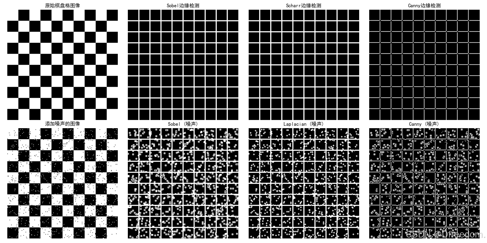
1. Sobel vs Scharr vs Canny

• Sobel: 边缘较粗，棋盘格线条有一定宽度
• Scharr: 与Sobel相似，但对角线边缘更清晰（旋转对称性更好）
• Canny: 产生单像素宽的边缘，最清晰

2. 抗噪性对比

• 干净图像: 所有算法都能检测出清晰的边缘
• 噪声图像:
  • Laplacian受噪声影响最大，出现大量误检测
  • Sobel/Scharr有一定抗噪性，但边缘变得模糊
  • Canny和LoG抗噪性最好，仍能保持主要边缘

观察要点解释：

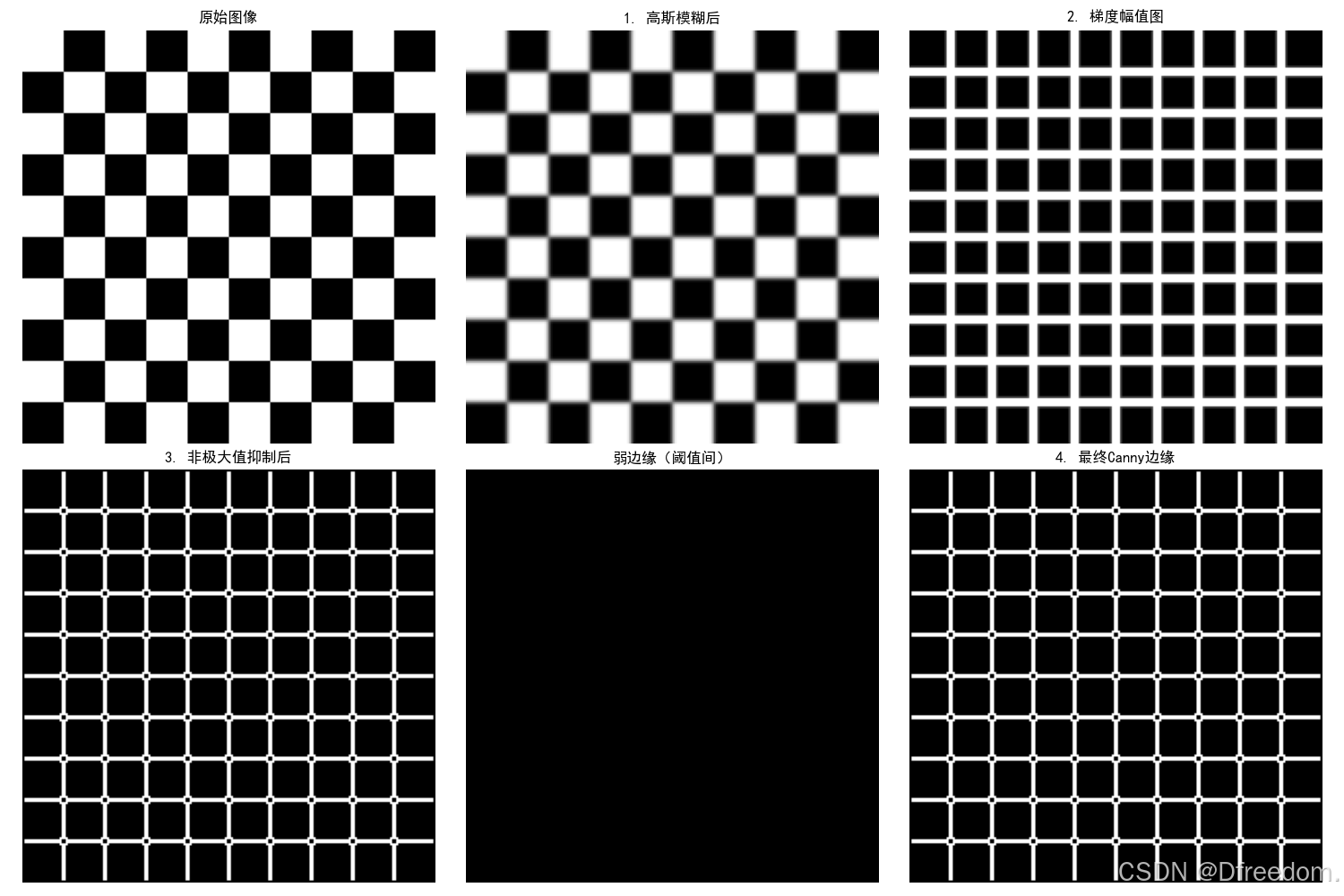
Canny算法步骤分解，代码中的visualize_canny_steps函数展示了：

• 原始图像​ → 清晰的棋盘格
• 高斯模糊后​ → 边缘稍微平滑
• 梯度幅值图​ → 边缘显示为亮带（粗边缘）
• 非极大值抑制后​ → 边缘细化
• 弱边缘​ → 阈值间的边缘点
• 最终Canny边缘​ → 单像素宽、连续的边缘

观察要点解释：

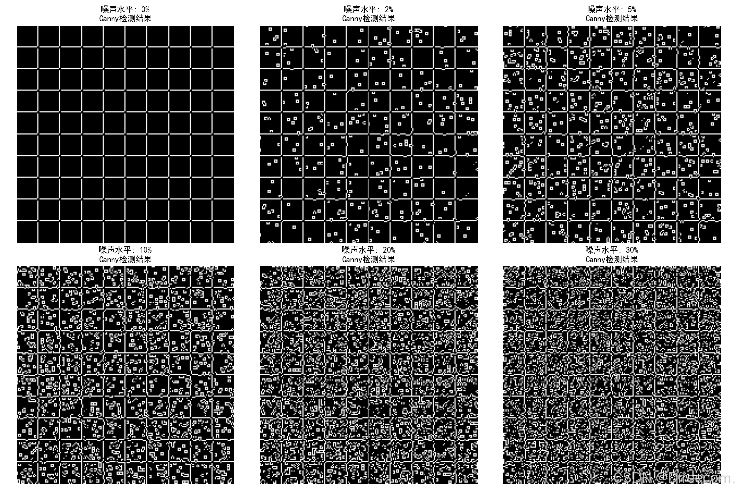
抗噪性测试，最后的抗噪性测试图展示了Canny算法在不同噪声水平下的表现：

• 噪声0%: 完美边缘
• 噪声2-5%: 边缘略有断裂但仍可识别
• 噪声10-20%: 开始出现噪声点，但主要边缘仍存在
• 噪声30%: 噪声点增多，但棋盘格结构仍可辨认

---