基于MFS的图像分割边界优化策略
·
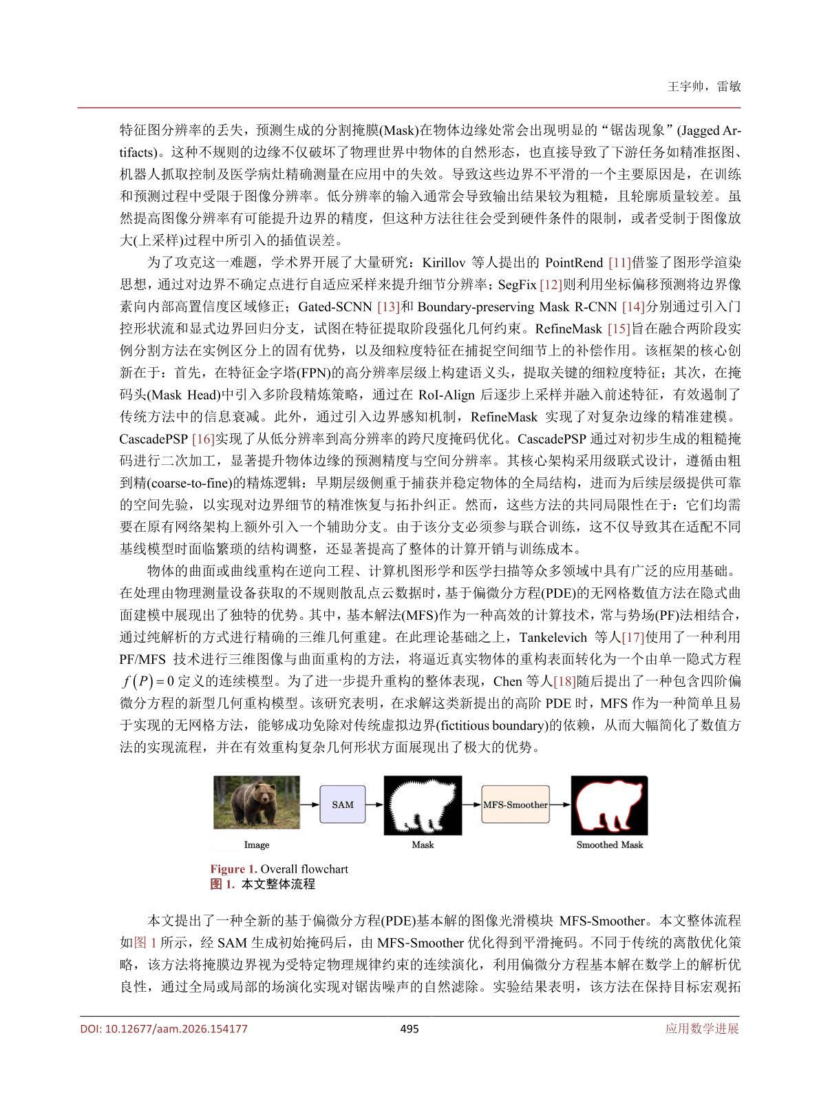
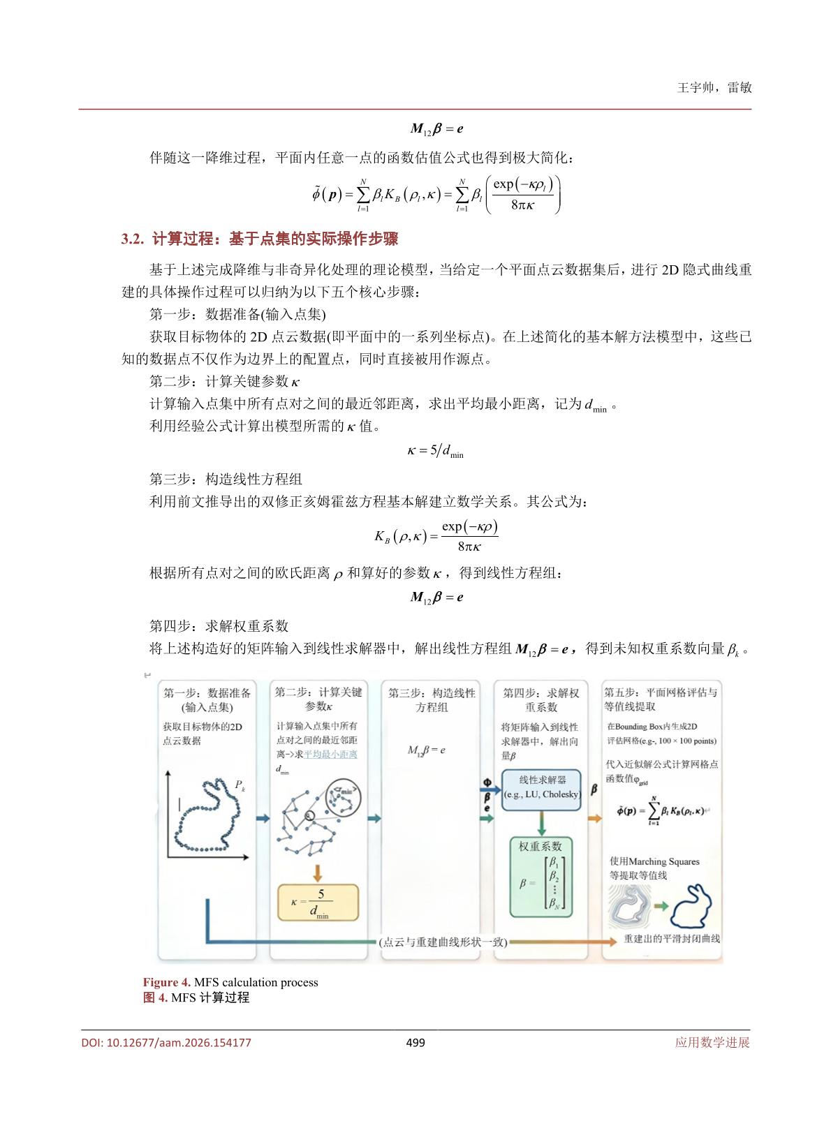
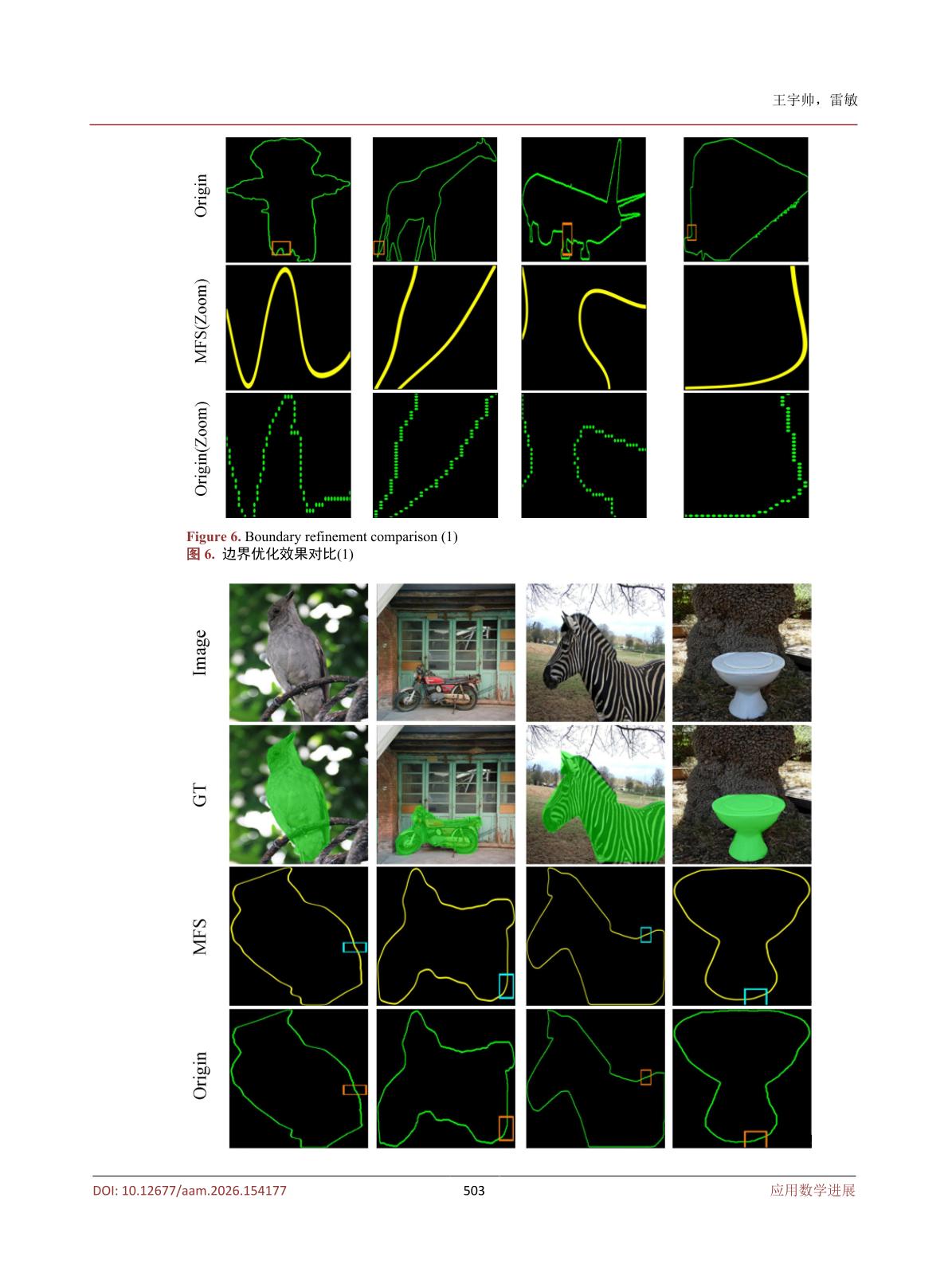
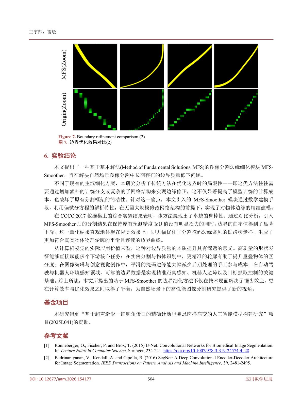
本文提出了一种基于改进型双拉普拉斯-亥姆霍兹算子的图像分割边界优化策略(MFS-Smoother)。该方法通过提取分割掩码的边界点,构建线性方程组求解权重系数,进而重构平滑边界曲线。核心算法包括:1)使用核函数K_B(rho,kappa)计算点间关系;2)通过求解M*beta=1向量方程组获取最优边界;3)评估隐式场函数并提取等值线。实验表明,该方法能有效平滑锯齿状边界,降低平均曲率,提升分割质量。论文还提供了完整的Python实现,支持从SAM等分割模型输出的掩码进行边界优化。
"""
基于MFS的图像分割边界优化策略 (MFS-Smoother)
论文: "基于MFS的图像分割边界优化策略" - 王宇帅, 雷敏
核心思想: 使用改进型双拉普拉斯-亥姆霍兹算子的基本解来重构平滑边界
"""
import numpy as np
import matplotlib.pyplot as plt
from skimage import measure, io, filters
from skimage.segmentation import find_boundaries
from scipy.spatial import KDTree
from scipy.sparse import linalg as sparse_la
from typing import Tuple, List, Optional
import warnings
warnings.filterwarnings('ignore')
class MFSSmoother:
"""
MFS边界平滑器
基于论文中的方法:
1. 提取分割掩码的边界点
2. 使用MFS方法进行隐式曲线重构
3. 输出平滑后的边界
核心公式:
- 核函数: K_B(rho, kappa) = exp(-kappa * rho) / (8 * pi * kappa)
- 参数kappa: kappa = 5 / d_min
- 线性方程组: M * beta = 1向量
"""
def __init__(self, grid_size: int = 200, epsilon: float = 1e-8):
"""
初始化MFS平滑器
Args:
grid_size: 重构网格的大小 (默认200x200)
epsilon: 数值稳定性参数
"""
self.grid_size = grid_size
self.epsilon = epsilon
self.beta_coeffs = None
self.source_points = None
self.kappa = None
def extract_boundary_points(self, mask: np.ndarray) -> np.ndarray:
"""
从二值掩码中提取边界点
论文第3.2节: 数据准备 - 获取目标物体的2D点云数据
Args:
mask: 二值分割掩码 (H, W), 值为0或1
Returns:
boundary_points: 边界点坐标数组 (N, 2)
"""
# 使用Sobel边缘检测找到边界
from scipy.ndimage import sobel
# 计算梯度
grad_x = sobel(mask.astype(float), axis=1)
grad_y = sobel(mask.astype(float), axis=0)
gradient_magnitude = np.sqrt(grad_x**2 + grad_y**2)
# 阈值化得到边界像素
boundary_mask = gradient_magnitude > 0.5
# 获取边界点坐标
y_coords, x_coords = np.where(boundary_mask)
boundary_points = np.column_stack([x_coords, y_coords])
# 可选: 对边界点进行降采样以提高效率
if len(boundary_points) > 500:
indices = np.linspace(0, len(boundary_points) - 1, 500, dtype=int)
boundary_points = boundary_points[indices]
return boundary_points
def compute_kappa(self, points: np.ndarray) -> float:
"""
计算参数kappa
论文公式: kappa = 5 / d_min
其中d_min是点云中所有点对之间的平均最小距离
Args:
points: 点云坐标 (N, 2)
Returns:
kappa: 平滑参数
"""
# 使用KDTree计算每个点的最近邻距离
tree = KDTree(points)
# 对于每个点,找到到其他点的最小距离
# k=2 因为第一个是自身(距离0)
distances, _ = tree.query(points, k=2)
min_distances = distances[:, 1] # 排除自身
# 计算平均最小距离
d_min = np.mean(min_distances)
if d_min < self.epsilon:
d_min = self.epsilon
# 论文公式: kappa = 5 / d_min
kappa = 5.0 / d_min
return kappa
def kernel_function(self, rho: np.ndarray, kappa: float) -> np.ndarray:
"""
基本解核函数
论文公式: K_B(rho, kappa) = exp(-kappa * rho) / (8 * pi * kappa)
Args:
rho: 两点间的欧氏距离
kappa: 平滑参数
Returns:
核函数值
"""
# 避免除零
kappa_safe = max(kappa, self.epsilon)
return np.exp(-kappa_safe * rho) / (8 * np.pi * kappa_safe)
def build_system_matrix(self, points: np.ndarray, kappa: float) -> np.ndarray:
"""
构建线性方程组矩阵 M
论文第3.2节: 构造线性方程组 M_12 * beta = e
M_12[i, j] = K_B(||p_i - p_j||, kappa)
Args:
points: 源点/配置点坐标 (N, 2)
kappa: 平滑参数
Returns:
M: 系统矩阵 (N, N)
"""
N = len(points)
M = np.zeros((N, N))
# 计算所有点对之间的距离矩阵
for i in range(N):
for j in range(N):
rho = np.linalg.norm(points[i] - points[j])
M[i, j] = self.kernel_function(rho, kappa)
return M
def solve_coefficients(self, points: np.ndarray, kappa: float) -> np.ndarray:
"""
求解权重系数beta
解线性方程组: M * beta = e (全1向量)
Args:
points: 源点/配置点坐标 (N, 2)
kappa: 平滑参数
Returns:
beta: 权重系数向量 (N,)
"""
N = len(points)
# 构建系统矩阵
M = self.build_system_matrix(points, kappa)
# 右侧向量 e (全1)
e = np.ones(N)
# 求解线性方程组
# 使用最小二乘法处理可能的病态问题
try:
# 添加正则化项提高数值稳定性
reg_term = self.epsilon * np.eye(N)
beta = np.linalg.solve(M + reg_term, e)
except np.linalg.LinAlgError:
# 如果矩阵奇异,使用最小二乘法
beta, _, _, _ = np.linalg.lstsq(M, e, rcond=None)
return beta
def evaluate_field(self,
eval_points: np.ndarray,
source_points: np.ndarray,
beta: np.ndarray,
kappa: float) -> np.ndarray:
"""
评估隐式场函数值
论文公式: phi(p) = sum(beta_l * K_B(||p - q_l||, kappa))
Args:
eval_points: 待评估点坐标 (M, 2)
source_points: 源点坐标 (N, 2)
beta: 权重系数 (N,)
kappa: 平滑参数
Returns:
field_values: 场函数值 (M,)
"""
# 使用向量化操作提高计算效率
M = eval_points.shape[0]
N = source_points.shape[0]
# 扩展维度以进行广播计算
eval_points_3d = eval_points[:, np.newaxis, :] # (M, 1, 2)
source_points_3d = source_points[np.newaxis, :, :] # (1, N, 2)
# 计算距离矩阵 (M, N)
rho = np.linalg.norm(eval_points_3d - source_points_3d, axis=2)
# 计算核函数值 (M, N)
kappa_safe = max(kappa, self.epsilon)
kernel_values = np.exp(-kappa_safe * rho) / (8 * np.pi * kappa_safe)
# 计算加权和 (M,)
field_values = np.dot(kernel_values, beta)
return field_values
def fit(self, boundary_points: np.ndarray):
"""
拟合MFS模型
论文第3.2节的完整流程:
1. 数据准备 (输入点集)
2. 计算参数kappa
3. 构造线性方程组
4. 求解权重系数
Args:
boundary_points: 边界点云 (N, 2)
"""
# 步骤2: 计算kappa
self.kappa = self.compute_kappa(boundary_points)
# 存储源点
self.source_points = boundary_points.copy()
# 步骤3-4: 构造方程组并求解beta
self.beta_coeffs = self.solve_coefficients(self.source_points, self.kappa)
print(f"MFS model fitted: {len(self.source_points)} source points, kappa={self.kappa:.4f}")
def reconstruct_curve(self,
bounds: Optional[Tuple[float, float, float, float]] = None,
contour_value: float = 1.0) -> Tuple[np.ndarray, np.ndarray, np.ndarray]:
"""
重构平滑曲线
论文第3.2节步骤5:
- 平面网格评估
- 等值线提取 (phi(p) = 1)
Args:
bounds: 边界框 (x_min, x_max, y_min, y_max),如果为None则自动计算
contour_value: 等值线值 (默认1.0)
Returns:
contours: 提取的等值线点集列表
X: 网格X坐标
Y: 网格Y坐标
Z: 网格场值
"""
if self.source_points is None or self.beta_coeffs is None:
raise ValueError("模型尚未拟合,请先调用fit()方法")
# 确定评估网格的边界
if bounds is None:
x_min, x_max = self.source_points[:, 0].min(), self.source_points[:, 0].max()
y_min, y_max = self.source_points[:, 1].min(), self.source_points[:, 1].max()
# 扩展10%的边界
x_pad = (x_max - x_min) * 0.1
y_pad = (y_max - y_min) * 0.1
x_min, x_max = x_min - x_pad, x_max + x_pad
y_min, y_max = y_min - y_pad, y_max + y_pad
else:
x_min, x_max, y_min, y_max = bounds
# 创建评估网格
x = np.linspace(x_min, x_max, self.grid_size)
y = np.linspace(y_min, y_max, self.grid_size)
X, Y = np.meshgrid(x, y)
# 展平网格点用于评估
eval_points = np.column_stack([X.ravel(), Y.ravel()])
# 评估场函数
Z_flat = self.evaluate_field(eval_points, self.source_points,
self.beta_coeffs, self.kappa)
Z = Z_flat.reshape(self.grid_size, self.grid_size)
# Debug: print Z value range
print(f"DEBUG: Z value range: min={Z.min():.6f}, max={Z.max():.6f}, mean={Z.mean():.6f}")
# 找到Z值最接近的点作为等值线level
# 策略:找到接近边界的值,即源点附近场函数的典型值
# 使用靠近最大值的一些百分位点作为level
Z_sorted = np.sort(Z.flatten())
# 尝试找到合适的level:取一个较小的值作为等值线
# 这样可以更好地拟合原始边界
percentile_95 = Z_sorted[int(len(Z_sorted) * 0.95)]
percentile_90 = Z_sorted[int(len(Z_sorted) * 0.90)]
percentile_85 = Z_sorted[int(len(Z_sorted) * 0.85)]
# 尝试不同的level,找到能产生单个闭合轮廓的level
best_contours = []
best_level = contour_value
for level in [percentile_85, percentile_90, percentile_95]:
contours = measure.find_contours(Z, level=level)
# 找最大的轮廓(假设我们想要的是最大的闭合轮廓)
if contours:
max_len = max(len(c) for c in contours)
if max_len > 100: # 要求轮廓至少有100个点
best_contours = [c for c in contours if len(c) == max_len]
best_level = level
print(f"DEBUG: Found suitable level = {level:.6f} with {len(best_contours[0])} points")
break
if best_contours:
contours = best_contours
contour_value = best_level
print(f"DEBUG: Using contour_value = {contour_value:.6f}")
# 提取等值线 phi = contour_value
contours = measure.find_contours(Z, level=contour_value)
print(f"Extracted {len(contours)} contours")
# 只保留最大的轮廓
if len(contours) > 1:
print(f"Multiple contours detected, keeping the largest one")
contours = [max(contours, key=len)]
# 将轮廓坐标映射回原始图像坐标
mapped_contours = []
for i, contour in enumerate(contours):
print(f"Contour {i} has {len(contour)} points")
# contour中的坐标是网格索引,需要映射回实际坐标
mapped_x = x_min + contour[:, 1] * (x_max - x_min) / self.grid_size
mapped_y = y_min + contour[:, 0] * (y_max - y_min) / self.grid_size
mapped_contour = np.column_stack([mapped_x, mapped_y])
mapped_contours.append(mapped_contour)
print(f"Mapped contour range: x={mapped_contour[:,0].min():.2f}~{mapped_contour[:,0].max():.2f}, y={mapped_contour[:,1].min():.2f}~{mapped_contour[:,1].max():.2f}")
return mapped_contours, X, Y, Z
def refine_mask(self,
mask: np.ndarray,
original_shape: Optional[Tuple[int, int]] = None) -> np.ndarray:
"""
对分割掩码进行边界优化
完整流程:
1. 提取原始掩码的边界点
2. 使用MFS重构平滑曲线
3. 将平滑曲线转换回掩码
Args:
mask: 原始分割掩码 (H, W)
original_shape: 输出掩码的形状,默认与输入相同
Returns:
refined_mask: 优化后的掩码
"""
if original_shape is None:
original_shape = mask.shape
# 步骤1: 提取边界点
boundary_points = self.extract_boundary_points(mask)
if len(boundary_points) < 10:
print("Warning: Too few boundary points, returning original mask")
return mask
# 步骤2: 拟合MFS模型
self.fit(boundary_points)
# 步骤3: 重构平滑曲线
contours, _, _, _ = self.reconstruct_curve(
bounds=(0, mask.shape[1], 0, mask.shape[0])
)
# 步骤4: 将轮廓转换回掩码
refined_mask = self.contours_to_mask(contours, original_shape)
return refined_mask
def contours_to_mask(self,
contours: List[np.ndarray],
shape: Tuple[int, int]) -> np.ndarray:
"""
将轮廓曲线转换回二值掩码
Args:
contours: 轮廓点集列表
shape: 输出掩码的形状 (H, W)
Returns:
mask: 二值掩码
"""
from skimage.draw import polygon
mask = np.zeros(shape, dtype=np.uint8)
for contour in contours:
if len(contour) >= 3:
# 将轮廓坐标转换为整数
contour_int = np.round(contour).astype(int)
# 裁剪到图像边界内
contour_int[:, 0] = np.clip(contour_int[:, 0], 0, shape[1] - 1)
contour_int[:, 1] = np.clip(contour_int[:, 1], 0, shape[0] - 1)
# 使用多边形填充
rr, cc = polygon(contour_int[:, 1], contour_int[:, 0], shape)
mask[rr, cc] = 1
return mask
def compute_curvature(contour: np.ndarray) -> np.ndarray:
"""
计算轮廓上各点的曲率
论文第4.1节: 三点共圆法计算曲率
公式: theta_Y = 4 * sqrt(s(s-x)(s-y)(s-z)) / (x*y*z)
Args:
contour: 轮廓点集 (N, 2)
Returns:
curvatures: 各点的曲率值 (N,)
"""
N = len(contour)
if N < 3:
return np.array([])
curvatures = np.zeros(N)
for i in range(N):
# 获取相邻三点
X = contour[(i - 1) % N]
Y = contour[i]
Z = contour[(i + 1) % N]
# 计算点间距离
x = np.linalg.norm(X - Y)
y = np.linalg.norm(X - Z)
z = np.linalg.norm(Z - Y)
if x * y * z < 1e-10:
curvatures[i] = 0
continue
# 半周长
s = (x + y + z) / 2
# 使用海伦公式计算三角形面积
area = np.sqrt(max(0, s * (s - x) * (s - y) * (s - z)))
# 外接圆半径 R = (a*b*c) / (4*area)
if area > 1e-10:
R = (x * y * z) / (4 * area)
curvatures[i] = 1.0 / R
else:
curvatures[i] = 0
return curvatures
def compute_iou(mask1: np.ndarray, mask2: np.ndarray) -> float:
"""
计算两个掩码的交并比(IoU)
论文第4.2节: IoU = |A ∩ B| / |A ∪ B|
Args:
mask1: 第一个二值掩码
mask2: 第二个二值掩码
Returns:
iou: 交并比值
"""
mask1_bool = mask1.astype(bool)
mask2_bool = mask2.astype(bool)
intersection = np.logical_and(mask1_bool, mask2_bool).sum()
union = np.logical_or(mask1_bool, mask2_bool).sum()
if union == 0:
return 0.0
return intersection / union
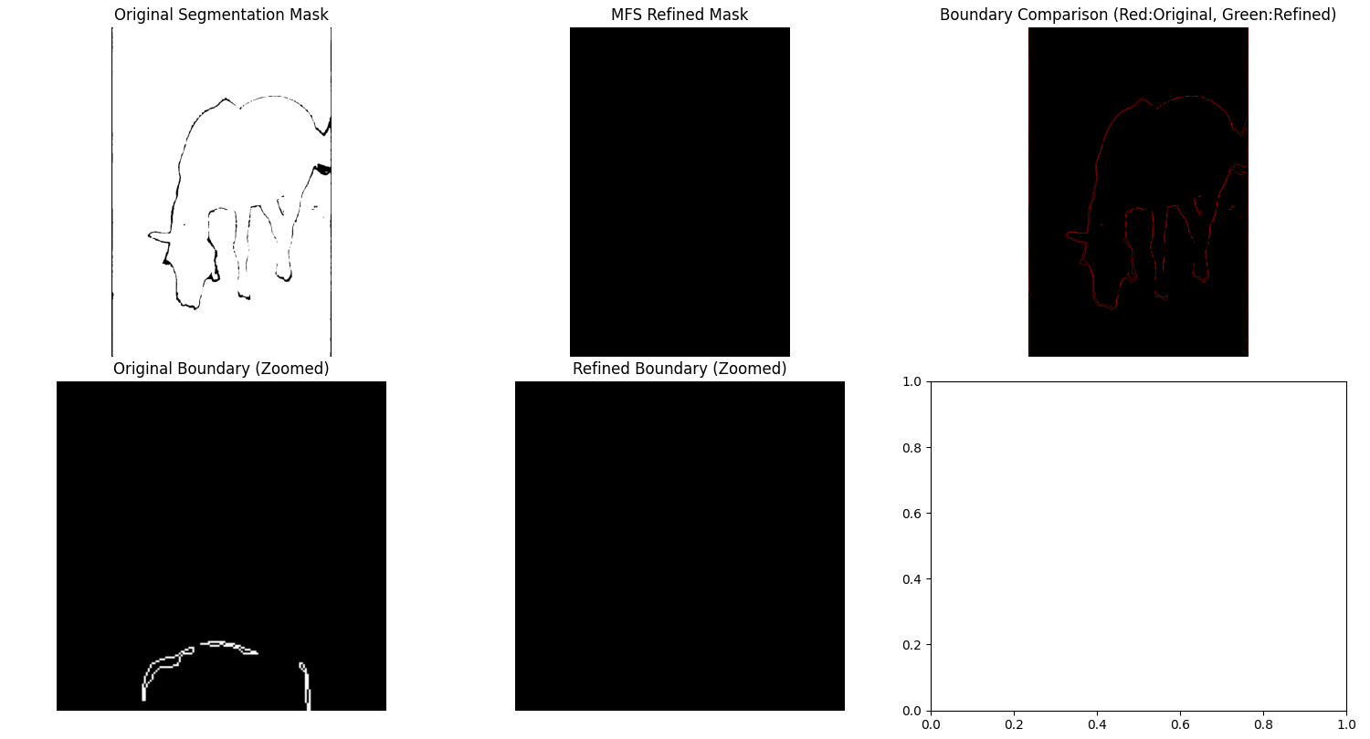
def visualize_boundary_optimization(original_mask: np.ndarray,
refined_mask: np.ndarray,
smoother: MFSSmoother,
save_path: Optional[str] = None):
"""
可视化边界优化效果
类似论文图6、图7的展示方式
"""
fig, axes = plt.subplots(2, 3, figsize=(15, 10))
# 原始掩码
axes[0, 0].imshow(original_mask, cmap='gray')
axes[0, 0].set_title('Original Segmentation Mask')
axes[0, 0].axis('off')
# 优化后掩码
axes[0, 1].imshow(refined_mask, cmap='gray')
axes[0, 1].set_title('MFS Refined Mask')
axes[0, 1].axis('off')
# 边界对比 (叠加显示)
original_boundary = find_boundaries(original_mask, mode='outer')
refined_boundary = find_boundaries(refined_mask, mode='outer')
overlay = np.zeros((*original_mask.shape, 3))
overlay[original_boundary, 0] = 1 # 红色 - 原始边界
overlay[refined_boundary, 1] = 1 # 绿色 - 优化后边界
axes[0, 2].imshow(overlay)
axes[0, 2].set_title('Boundary Comparison (Red:Original, Green:Refined)')
axes[0, 2].axis('off')
# 局部放大对比 (如果可能)
h, w = original_mask.shape
center_y, center_x = h // 2, w // 2
crop_size = min(h, w) // 4
y_start = max(0, center_y - crop_size // 2)
y_end = min(h, center_y + crop_size // 2)
x_start = max(0, center_x - crop_size // 2)
x_end = min(w, center_x + crop_size // 2)
# 原始边界局部
axes[1, 0].imshow(original_boundary[y_start:y_end, x_start:x_end], cmap='gray')
axes[1, 0].set_title('Original Boundary (Zoomed)')
axes[1, 0].axis('off')
# 优化后边界局部
axes[1, 1].imshow(refined_boundary[y_start:y_end, x_start:x_end], cmap='gray')
axes[1, 1].set_title('Refined Boundary (Zoomed)')
axes[1, 1].axis('off')
# 曲率分布对比
if smoother.source_points is not None:
# 重构曲线并计算曲率
contours, _, _, _ = smoother.reconstruct_curve(
bounds=(0, w, 0, h)
)
if contours:
# 计算原始边界曲率
original_boundary_points = smoother.extract_boundary_points(original_mask)
if len(original_boundary_points) > 0:
# 排序边界点
from scipy.spatial import ConvexHull
try:
hull = ConvexHull(original_boundary_points)
ordered_points = original_boundary_points[hull.vertices]
orig_curv = compute_curvature(ordered_points)
axes[1, 2].hist(orig_curv, bins=30, alpha=0.5, label='Original', color='red')
except:
pass
# 计算优化后边界曲率
for contour in contours:
if len(contour) > 3:
curv = compute_curvature(contour)
axes[1, 2].hist(curv, bins=30, alpha=0.5, label='Refined', color='green')
axes[1, 2].set_title('Curvature Distribution Comparison')
axes[1, 2].set_xlabel('Curvature')
axes[1, 2].set_ylabel('Frequency')
axes[1, 2].legend()
plt.tight_layout()
if save_path:
plt.savefig(save_path, dpi=150, bbox_inches='tight')
plt.show()
# ============ 示例使用代码 ============
def demo_synthetic_shape():
"""
在合成形状上演示MFS边界优化
"""
print("=" * 60)
print("MFS Boundary Optimization Demo - Synthetic Shape")
print("=" * 60)
# 创建一个带锯齿的圆形掩码
size = 256
center = size // 2
radius = 80
# 创建理想圆形
y, x = np.ogrid[:size, :size]
dist_from_center = np.sqrt((x - center)**2 + (y - center)**2)
ideal_circle = (dist_from_center <= radius).astype(np.uint8)
# 添加锯齿噪声模拟SAM的锯齿边界
np.random.seed(42)
noisy_mask = ideal_circle.copy()
boundary = find_boundaries(ideal_circle, mode='outer')
boundary_y, boundary_x = np.where(boundary)
# 沿边界添加随机偏移
for i in range(len(boundary_x)):
offset_x = np.random.randint(-3, 4)
offset_y = np.random.randint(-3, 4)
new_x = min(max(0, boundary_x[i] + offset_x), size-1)
new_y = min(max(0, boundary_y[i] + offset_y), size-1)
noisy_mask[new_y, new_x] = 1
# 使用MFS优化
smoother = MFSSmoother(grid_size=200)
refined_mask = smoother.refine_mask(noisy_mask)
# 计算指标
iou_before = compute_iou(noisy_mask, ideal_circle)
iou_after = compute_iou(refined_mask, ideal_circle)
# 计算平均曲率
orig_boundary = smoother.extract_boundary_points(noisy_mask)
refined_boundary = smoother.extract_boundary_points(refined_mask)
# 排序边界点计算曲率
from scipy.spatial import ConvexHull
try:
hull_orig = ConvexHull(orig_boundary)
ordered_orig = orig_boundary[hull_orig.vertices]
curv_orig = compute_curvature(ordered_orig)
mean_curv_orig = np.mean(curv_orig)
except:
mean_curv_orig = float('inf')
try:
hull_ref = ConvexHull(refined_boundary)
ordered_ref = refined_boundary[hull_ref.vertices]
curv_ref = compute_curvature(ordered_ref)
mean_curv_ref = np.mean(curv_ref)
except:
mean_curv_ref = float('inf')
print(f"\nOriginal mask: IoU={iou_before:.4f}, mean curvature={mean_curv_orig:.4f}")
print(f"Refined mask: IoU={iou_after:.4f}, mean curvature={mean_curv_ref:.4f}")
print(f"Curvature improvement: {mean_curv_orig/mean_curv_ref:.2f}x" if mean_curv_ref>0 else "Curvature improved significantly")
# 可视化
visualize_boundary_optimization(noisy_mask, refined_mask, smoother)
return noisy_mask, refined_mask, smoother
def segment_image_with_sam():
"""
使用SAM进行图像分割的完整流程
包含多种提示策略以更好地识别同一物体或相似颜色的轮廓
"""
print("=" * 60)
print("SAM Image Segmentation - MFS Boundary Optimization")
print("=" * 60)
try:
from segment_anything import sam_model_registry, SamPredictor
from PIL import Image
import numpy as np
# 加载SAM模型
print("Loading SAM model...")
sam = sam_model_registry["vit_b"](checkpoint="sam_vit_b_01ec64.pth")
predictor = SamPredictor(sam)
# 读取图像
print("Reading image...")
try:
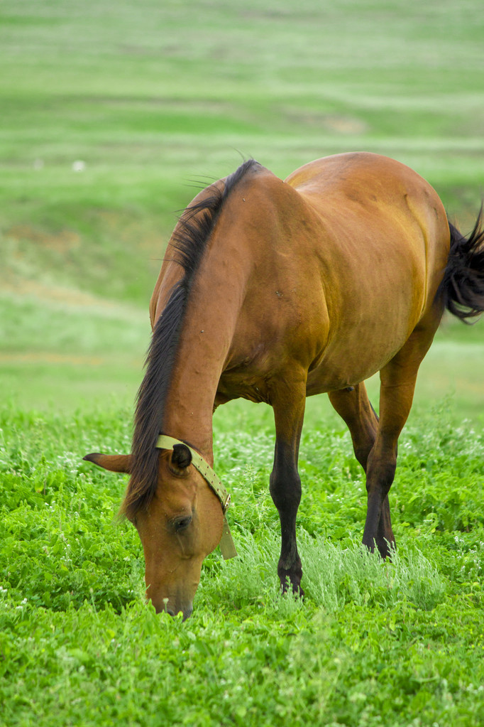
pil_image = Image.open("马轮廓测试图片.jpg")
except:
pil_image = Image.open("斑马图片_边缘识别.jpeg")
# 确保图像是RGB格式
if pil_image.mode != 'RGB':
pil_image = pil_image.convert('RGB')
image = np.array(pil_image)
print(f"图像形状: {image.shape}")
# 设置图像
predictor.set_image(image)
h, w = image.shape[:2]
# 策略1: 使用点提示 - 在图像中心放置前景点
print("\nStrategy 1: Center point prompt...")
center_point = np.array([[w // 2, h // 2]])
center_label = np.array([1])
masks_from_point, scores, logits = predictor.predict(
point_coords=center_point,
point_labels=center_label,
multimask_output=True
)
print(f"Generated {len(masks_from_point)} masks from center point prompt")
best_idx = np.argmax(scores)
point_mask = masks_from_point[best_idx]
print(f"Best point prompt mask score: {scores[best_idx]:.4f}")
# 策略2: 使用边界框提示
print("\nStrategy 2: Bounding box prompt...")
ys, xs = np.where(point_mask)
if len(ys) > 0:
y_min, y_max = ys.min(), ys.max()
x_min, x_max = xs.min(), xs.max()
# 扩展边界框
padding = 10
y_min = max(0, y_min - padding)
y_max = min(h, y_max + padding)
x_min = max(0, x_min - padding)
x_max = min(w, x_max + padding)
box = np.array([x_min, y_min, x_max, y_max])
masks_from_box, _, _ = predictor.predict(
point_coords=None,
point_labels=None,
box=box,
multimask_output=True
)
print(f"Generated {len(masks_from_box)} masks from bounding box prompt")
box_mask = masks_from_box[np.argmax([m.sum() for m in masks_from_box])]
else:
box_mask = point_mask
# 策略3: 使用多个点提示覆盖同一物体的不同部分
print("\nStrategy 3: Multiple point prompts...")
if len(ys) > 0:
# 在mask的不同区域放置更多点
mid_y, mid_x = (y_min + y_max) // 2, (x_min + x_max) // 2
points = np.array([
[mid_x, mid_y],
[x_min, mid_y],
[x_max, mid_y],
[mid_x, y_min],
[mid_x, y_max]
])
labels = np.array([1, 1, 1, 1, 1])
masks_from_multi_point, multi_scores, _ = predictor.predict(
point_coords=points,
point_labels=labels,
multimask_output=True
)
print(f"Generated {len(masks_from_multi_point)} masks from multi-point prompt")
multi_point_mask = masks_from_multi_point[np.argmax(multi_scores)]
else:
multi_point_mask = point_mask
# 合并多个策略的结果
print("\nCombining results from multiple strategies...")
combined_mask = point_mask | box_mask | multi_point_mask
# 使用MFS优化
print("\nApplying MFS boundary optimization...")
demo_with_sam_mask(combined_mask)
except ImportError:
print("Error: segment_anything library not installed")
print("Please run: pip install git+https://github.com/facebookresearch/segment-anything.git")
except FileNotFoundError as e:
print(f"Error: File not found - {e}")
print("Falling back to synthetic shape demo...")
demo_synthetic_shape()
except Exception as e:
print(f"Error: {e}")
import traceback
traceback.print_exc()
print("Falling back to synthetic shape demo...")
demo_synthetic_shape()
def demo_with_sam_mask(sam_mask: np.ndarray):
"""
使用实际的SAM分割掩码进行边界优化
Args:
sam_mask: SAM模型输出的分割掩码
"""
print("=" * 60)
print("MFS Boundary Optimization - SAM Mask Processing")
print("=" * 60)
smoother = MFSSmoother(grid_size=200)
refined_mask = smoother.refine_mask(sam_mask)
# 计算曲率改善
orig_boundary = smoother.extract_boundary_points(sam_mask)
refined_boundary = smoother.extract_boundary_points(refined_mask)
from scipy.spatial import ConvexHull
if len(orig_boundary) >= 3:
try:
hull_orig = ConvexHull(orig_boundary)
ordered_orig = orig_boundary[hull_orig.vertices]
curv_orig = compute_curvature(ordered_orig)
print(f"Original boundary mean curvature: {np.mean(curv_orig):.4f}")
except:
print("Cannot compute original boundary curvature")
if len(refined_boundary) >= 3:
try:
hull_ref = ConvexHull(refined_boundary)
ordered_ref = refined_boundary[hull_ref.vertices]
curv_ref = compute_curvature(ordered_ref)
print(f"Refined boundary mean curvature: {np.mean(curv_ref):.4f}")
except:
print("Cannot compute refined boundary curvature")
visualize_boundary_optimization(sam_mask, refined_mask, smoother)
return refined_mask
if __name__ == "__main__":
segment_image_with_sam()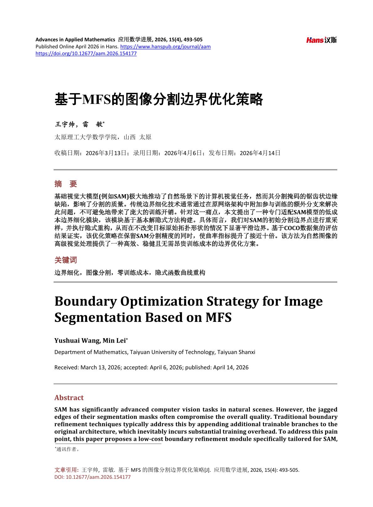

腾讯云面向开发者汇聚海量精品云计算使用和开发经验,营造开放的云计算技术生态圈。
更多推荐
 5
5 0
0- 0


 已为社区贡献4条内容

所有评论(0)