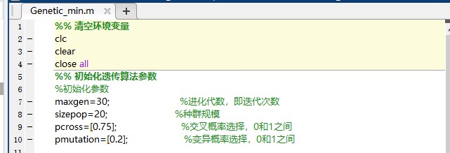
bp神经网络遗传算法寻优代码模型，注释清楚，可以运行，

最近在研究优化算法，发现BP神经网络结合遗传算法来寻优真的超有趣！今天就来给大家分享一下相关的代码模型，并且穿插着讲讲其中的门道。

首先呢，我们来看一下整体的代码框架。这里用Python来实现，先导入必要的库：

import numpy as np
import matplotlib.pyplot as plt
import random

numpy用于数值计算，matplotlib用来绘图，random则是为了生成随机数，方便后续遗传算法中的一些操作。

接下来定义BP神经网络的结构和相关参数：

# 定义输入层、隐藏层和输出层的节点数
input_layer_size = 2
hidden_layer_size = 3
output_layer_size = 1

# 学习率
alpha = 0.1

这里我们设置输入层有2个节点，隐藏层有3个节点，输出层有1个节点，学习率为0.1。学习率控制着每次权重更新的幅度，太小会导致收敛慢，太大可能会错过最优解。

然后是BP神经网络的前向传播函数：

def sigmoid(z):
    return 1 / (1 + np.exp(-z))


def forward_propagation(X, theta1, theta2):
    a1 = np.hstack([np.ones((X.shape[0], 1)), X])
    z2 = a1.dot(theta1.T)
    a2 = sigmoid(z2)
    a2 = np.hstack([np.ones((a2.shape[0], 1)), a2])
    z3 = a2.dot(theta2.T)
    h = sigmoid(z3)
    return h, a1, z2, a2, z3

sigmoid函数是BP神经网络中常用的激活函数，它能将输入值映射到0到1之间。forward_propagation函数实现了前向传播的过程，从输入层经过隐藏层到输出层，依次计算每个节点的输出。

接着是计算代价函数（这里用均方误差）：

def cost_function(X, y, theta1, theta2):
    m = X.shape[0]
    h, _, _, _, _ = forward_propagation(X, theta1, theta2)
    J = (1 / (2 * m)) * np.sum((h - y) ** 2)
    return J

代价函数衡量了预测值与真实值之间的误差，我们希望通过优化权重来使代价函数最小化。

再来看反向传播函数，这可是BP神经网络的核心：

def back_propagation(X, y, theta1, theta2, h, a1, z2, a2, z3):
    m = X.shape[0]
    delta3 = h - y
    delta2 = delta3.dot(theta2) * (a2 * (1 - a2))
    delta2 = delta2[:, 1:]
    theta1_grad = (1 / m) * delta2.T.dot(a1)
    theta2_grad = (1 / m) * delta3.T.dot(a2)
    return theta1_grad, theta2_grad

反向传播通过计算误差的梯度，来更新权重。这里根据输出层和隐藏层的误差，逐步计算出对权重的梯度。

然后是更新权重的函数：

def update_weights(theta1, theta2, theta1_grad, theta2_grad):
    theta1 = theta1 - alpha * theta1_grad
    theta2 = theta2 - alpha * theta2_grad
    return theta1, theta2

根据梯度和学习率来更新权重。

现在进入遗传算法部分。首先初始化种群：

# 初始化种群
def initialize_population(population_size, theta1_size, theta2_size):
    population = []
    for _ in range(population_size):
        theta1 = np.random.rand(hidden_layer_size, input_layer_size + 1)
        theta2 = np.random.rand(output_layer_size, hidden_layer_size + 1)
        population.append([theta1, theta2])
    return population

随机生成一定数量的权重组合作为初始种群。

然后是计算适应度函数，这里用代价函数来衡量：

def fitness_function(population, X, y):
    fitness = []
    for individual in population:
        theta1, theta2 = individual
        J = cost_function(X, y, theta1, theta2)
        fitness.append(1 / J)  # 因为要最大化适应度，所以用1/代价函数
    return fitness

适应度越高表示个体越优。

接着是选择操作，这里用轮盘赌选择：

def roulette_wheel_selection(population, fitness):
    total_fitness = sum(fitness)
    selection_probabilities = [fit / total_fitness for fit in fitness]
    selected_index = np.random.choice(len(population), p=selection_probabilities)
    return population[selected_index]

轮盘赌选择根据个体的适应度比例来选择个体。

交叉操作：

def crossover(parent1, parent2):
    theta1_crossover_point = random.randint(0, parent1[0].shape[0] - 1)
    theta2_crossover_point = random.randint(0, parent1[1].shape[0] - 1)
    child1_theta1 = np.vstack([parent1[0][:theta1_crossover_point, :], parent2[0][theta1_crossover_point:, :]])
    child1_theta2 = np.vstack([parent1[1][:theta2_crossover_point, :], parent2[1][theta2_crossover_point:, :]])
    child2_theta1 = np.vstack([parent2[0][:theta1_crossover_point, :], parent1[0][theta1_crossover_point:, :]])
    child2_theta2 = np.vstack([parent2[1][:theta2_crossover_point, :], parent1[1][theta2_crossover_point:, :]])
    return [child1_theta1, child1_theta2], [child2_theta1, child2_theta2]

交叉操作交换父母个体的部分权重信息。

变异操作：

def mutation(individual, mutation_rate):
    theta1, theta2 = individual
    for i in range(theta1.shape[0]):
        for j in range(theta1.shape[1]):
            if random.random() < mutation_rate:
                theta1[i, j] = np.random.rand()
    for i in range(theta2.shape[0]):
        for j in range(theta2.shape[1]):
            if random.random() < mutation_rate:
                theta2[i, j] = np.random.rand()
    return [theta1, theta2]

变异操作以一定概率随机改变权重值，防止算法陷入局部最优。

最后是遗传算法的主循环：

# 遗传算法主循环
def genetic_algorithm(X, y, population_size, generations, mutation_rate):
    population = initialize_population(population_size, (hidden_layer_size, input_layer_size + 1),
                                       (output_layer_size, hidden_layer_size + 1))
    best_fitness = -np.inf
    best_individual = None
    for gen in range(generations):
        fitness = fitness_function(population, X, y)
        for i in range(population_size // 2):
            parent1 = roulette_wheel_selection(population, fitness)
            parent2 = roulette_wheel_selection(population, fitness)
            child1, child2 = crossover(parent1, parent2)
            child1 = mutation(child1, mutation_rate)
            child2 = mutation(child2, mutation_rate)
            population[i * 2] = child1
            population[i * 2 + 1] = child2
        current_best_fitness = max(fitness)
        if current_best_fitness > best_fitness:
            best_fitness = current_best_fitness
            best_individual = population[np.argmax(fitness)]
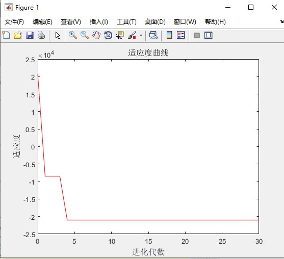
        print(f"Generation {gen}: Best Fitness = {best_fitness}")
    return best_individual

在主循环中，不断进行选择、交叉和变异操作，更新种群，最终找到最优的权重组合。

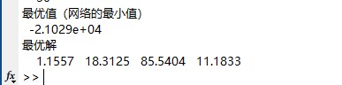
完整的代码运行起来后，就能通过BP神经网络结合遗传算法来对给定的数据进行寻优啦！

通过这样的代码模型，我们可以看到BP神经网络和遗传算法是如何相互协作，一步步找到最优解的。是不是很神奇？希望这篇分享能让大家对这个有趣的优化算法组合有更清晰的了解！

以上就是今天的全部内容啦，代码中的每一步都是为了实现更好的寻优效果，大家可以根据实际需求调整参数，进一步探索这个模型的魅力！